Harmonic-balance stability

hbstability analyzes the local stability of a harmonic balance operating point: it finds the temporal poles of the circuit linearized about it. A pole with a positive real part describes a perturbation that grows. Pass nonlinear=pump to analyze a computed biased or pumped orbit; without an operating point, junctions are linearized about zero phase.

A converged HB solution need not be stable. hblinsolve can still return finite small-signal gain beyond a parametric threshold. Pole analysis reveals the growing perturbation, as shown in a paramp through its threshold.

This is a local stability analysis of a periodic operating point. It accepts one fundamental angular frequency. Express commensurate drives as harmonics of that fundamental; an HB solution with several independent frequency axes is not accepted. A quasiperiodic operating point has no single pump period for this analysis.

Choose a method

Method	Use it for	Returned poles
Monodromy(), the default	Pumped circuits with a time-domain realization, including transmission-line delays	Up to nev least damped numerically resolved modes, 10 by default, with one frequency representative per mode
DenseSpectrum()	A reference calculation for a small polynomial problem	Every accepted finite pole of the harmonic truncation, including Floquet aliases
ShiftInvert(shifts; nev)	Modes near specified complex frequencies	Up to nev poles per shift; a local search can miss instabilities elsewhere
ContourIntegral(center, radius)	Exact unpumped delays, LaplaceResponse models, or a bounded spectral region	Accepted poles inside the circle, subject to numerical completeness checks

Without a pump, Monodromy() uses DenseSpectrum() instead of a period map. That fallback has a default limit of 1000 unknowns; use an explicit method to change the limit or search a larger problem. Unpumped exact delays and LaplaceResponse models require ContourIntegral().

A shift 1e6 + im*2pi*f searches near the frequency f in Hz, a little to the right of the axis so as not to sit on a marginal pole. Frequencies passed to the API are angular frequencies in rad/s; real(s) is a growth or decay rate in inverse seconds. A stable mode's amplitude decay time is -1/real(s), and its frequency in Hz is imag(s)/(2pi) for the chosen Floquet representative.

Choose accuracy and output controls

Control	What it changes	How to check it
Pump harmonics in hbnlsolve	The HB orbit and the linearization about it, for every method	Recompute the operating point with more harmonics, then repeat the stability analysis
Monodromy(steps=N)	Time discretization of the orbit and period map; also sampling of profiles and line histories	Repeat the full solve at 2N, and again if the rates have not settled
Nmodulationharmonics=(H,) with Monodromy	The exported profile window around each mode's chosen frequency; it does not truncate the map eigenproblem	Widen the window to capture the profile; require 2H + 1 <= steps
Nmodulationharmonics=(H,) with a polynomial/contour method	The harmonic truncation of the perturbation eigenproblem	Increase H and compare matched poles and profiles
Monodromy(nev=k) or nev=:all	How many resolved modes are returned, and among which rateerrors follows mode mixing	Increase it to inspect more modes and, in a crowded spectrum, to check the rate errors' sensitivity to omitted modes; it does not improve timestep accuracy or remove the dense eigensolve
Method tolerances and search settings	Accuracy and coverage of the finite eigenproblem	Check converged, residuals, and searches; these do not replace orbit/discretization refinement

Compare changes in real parts against the growth or decay rates, not against a GHz oscillation frequency. The returned rateerrors is an estimate of each rate's timestep error for pumped Monodromy, from the map at twice the steps; it is not a certified error bound or a substitute for the full refinement above. edgeweights measures profile content at the outer harmonics. A small value does not bound the error in a pole. See Interpreting accuracy for the separate checks.

A pumped JPA

The current-pumped JPA, its operating point first:

using JosephsonCircuits

circuit = Circuit([
    (:p, 1, 0, Port(1; Z0 = 50.0)),
    (:cc, 1, 2, Capacitor(100e-15)),
    (:jj, 2, 0, JosephsonJunction(1e-9)),
    (:cj, 2, 0, Capacitor(1e-12)),
])
wp = (2pi*4.75001e9,)
sources = [(mode = (1,), port = 1, current = 0.00565e-6)]
pump = hbnlsolve(wp, (16,), sources, circuit)
@assert pump.solverinfo.converged

The default period map returns this circuit's two resolved modes. Larger circuits return at most 10 by default; Monodromy(nev=:all) requests all numerically resolved modes:

modes = hbstability(circuit; nonlinear = pump)
@assert modes.converged && length(modes.poles) == 2
round.(modes.poles; sigdigits = 6)

2-element Vector{ComplexF64}:
 -3.93277e7 + 2.98452e10im
 -3.58595e8 + 2.98452e10im

Both decay, in about 25 ns and 2.8 ns. The polynomial in the harmonics of the pump, with four harmonics of the perturbation either side, finds the same two near the pump frequency:

shift = 1e6 + im*wp[1]
coarse = hbstability(circuit; nonlinear = pump, Nmodulationharmonics = (4,),
    method = ShiftInvert(shift; nev = 2))
moved(a, b) = maximum(minimum(abs.(b.poles .- s)) for s in a.poles)
@assert coarse.converged && moved(modes, coarse) < 1e-4*maximum(abs, modes.poles)
round.(coarse.poles; sigdigits = 6)

2-element Vector{ComplexF64}:
 -3.93279e7 + 2.98452e10im
 -3.58595e8 + 2.98452e10im

Their convergence is checked by solving with more of what each method truncates, the harmonics of the perturbation and of the pump, and the steps of the period: the poles barely move, and the weight of the outermost harmonics, edgeweights, falls. The rates are compared with the rates themselves, since a change far below a pole's frequency can still move a small rate across zero. The period map also returns rateerrors, an estimate from the selected modes propagated together at twice the steps, scaled to the coarse map's error at the rule's fourth order. In this example it agrees with the error found against a map at sixteen times the steps. That agreement is checked here; it is not guaranteed for another circuit.

refined = hbstability(circuit; nonlinear = pump, Nmodulationharmonics = (6,),
    method = ShiftInvert(shift; nev = 2))
pump20 = hbnlsolve(wp, (20,), sources, circuit)
pumpcheck = hbstability(circuit; nonlinear = pump20, Nmodulationharmonics = (6,),
    method = ShiftInvert(shift; nev = 2))
steps = hbstability(circuit; nonlinear = pump, method = Monodromy(steps = 1024))
rates(r) = sort(real.(r.poles))
@assert refined.converged && pumpcheck.converged
@assert moved(coarse, refined) < 10 && moved(refined, pumpcheck) < 10
@assert maximum(abs, rates(steps) .- rates(modes)) < 1e-4*minimum(abs, rates(modes))
@assert isapprox(maximum(modes.rateerrors), maximum(abs, rates(steps) .- rates(modes)); rtol = 0.01)
(harmonics = moved(coarse, refined), pump = moved(refined, pumpcheck),
    steps = maximum(abs, rates(steps) .- rates(modes)), estimate = maximum(modes.rateerrors),
    edgeweights = (maximum(coarse.edgeweights), maximum(refined.edgeweights)))

(harmonics = 0.6026400023521558, pump = 1.9788742065429688e-5, steps = 239.39765632897615, estimate = 239.05453202387523, edgeweights = (5.25774852318e-6, 2.986895528626287e-11))

A paramp through its threshold

A junction biased at half its critical current mixes three waves, and pumped through its port at twice its biased resonance it amplifies. Below its threshold the gain at the center of its band follows from its two poles there: a resonator whose poles are -κ/2 ± g reflects with the gain ((κ²/4 + g²)/(κ²/4 - g²))², which in the poles' real parts is ((s₁² + s₂²)/(2s₁s₂))². The resonance is a pole of the unpumped operating point:

using JosephsonCircuits

Lj = 1e-9
circuit = Circuit([
    (:p1, 1, 0, Port(1; Z0 = 50.0)),
    (:cc, 1, 2, Capacitor(100e-15)),
    (:jj, 2, 0, JosephsonJunction(Lj)),
    (:cj, 2, 0, Capacitor(1e-12)),
    (:p2, 2, 0, Port(2; Z0 = 1e6)),
])
bias = (mode = (0,), port = 2, current = LjtoIc(Lj)/2)
static = hbnlsolve((2pi*5e9,), (8,), [bias], circuit; dc = true, odd = true, even = true)
w0 = maximum(imag, hbstability(circuit; nonlinear = static, Nmodulationharmonics = (0,)).poles)
w0/(2pi*1e9)

4.4691894168742765

The peak gain hblinsolve finds near the resonance, the gain the two modes there predict, and the least damped mode's rate, as the pump grows:

ws = collect(range(w0 - 2pi*200e6, w0 + 2pi*200e6; length = 400))
currents = [20e-9, 40e-9, 60e-9, 80e-9, 100e-9]
results = map(currents) do Ip
    sources = [bias, (mode = (1,), port = 1, current = Ip)]
    pump = hbnlsolve((2w0,), (16,), sources, circuit; dc = true, odd = true, even = true)
    lin = hblinsolve(ws, circuit; nonlinear = pump, Nmodulationharmonics = (6,),
        threewavemixing = true, fourwavemixing = true, keyedarrays = false)
    k = lin.signalindex
    spectrum = hbstability(circuit; nonlinear = pump)
    @assert pump.solverinfo.converged && spectrum.converged
    s1, s2 = real.(spectrum.poles[1:2])
    (spectrum = spectrum, gain = 10log10(maximum(abs2, lin.S[k, k, :])), rate = s1,
        frompoles = s1 < 0 ? 10log10(((s1^2 + s2^2)/(2s1*s2))^2) : NaN)
end
@assert all(abs(r.gain - r.frompoles) < 0.2 for r in results if r.rate < 0)
@assert results[1].rate < 0 < results[end].rate
[(pump = "$(round(Int, Ip*1e9)) nA", hblinsolve = round(r.gain; digits = 2),
    frompoles = r.rate < 0 ? round(r.frompoles; digits = 2) : "unstable",
    rate = round(r.rate; sigdigits = 3)) for (Ip, r) in zip(currents, results)]

5-element Vector{NamedTuple{(:pump, :hblinsolve, :frompoles, :rate)}}:
 (pump = "20 nA", hblinsolve = 1.45, frompoles = 1.49, rate = -1.25e8)
 (pump = "40 nA", hblinsolve = 6.15, frompoles = 6.18, rate = -7.35e7)
 (pump = "60 nA", hblinsolve = 17.55, frompoles = 17.65, rate = -2.18e7)
 (pump = "80 nA", hblinsolve = 16.18, frompoles = "unstable", rate = 2.97e7)
 (pump = "100 nA", hblinsolve = 8.85, frompoles = "unstable", rate = 8.12e7)

Between 60 and 80 nA the least damped pole crosses into the right half plane. Past it the operating point still converges and hblinsolve still returns a gain, 16 dB at 80 nA, the response of a linearization about an orbit that does not persist:

using Plots
plot(currents .* 1e9, [r.rate for r in results] ./ 1e6; marker = :circle,
    xlabel = "Pump current (nA)", ylabel = "Least damped rate (1/μs)",
    label = "hbstability", legend = :topleft, size = (620, 360), color = :royalblue)
hline!([0]; color = :gray, linestyle = :dash, label = "")
plot!(twinx(), currents .* 1e9, [r.gain for r in results]; marker = :square,
    ylabel = "Peak gain (dB)", label = "hblinsolve", legend = :topright,
    color = :darkorange)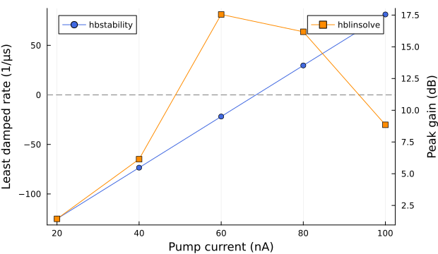

Track a mode through the sweep

Results are sorted by growth rate at each parameter value. A mode's array index can change when two rates cross. Track its profile with JosephsonCircuits.matchpoles, reusing the spectra just computed:

tracked, overlaps = let
    poles = [results[1].spectrum.poles[1]]
    overlaps = [1.0]
    index = 1
    for j in 2:length(results)
        previous, current = results[j-1].spectrum, results[j].spectrum
        match = only(JosephsonCircuits.matchpoles(previous, current; indices = [index]))
        match.index != 0 || error("Unmatched mode: reduce the pump-current spacing or return more candidate modes.")
        index = match.index
        push!(poles, current.poles[index])
        push!(overlaps, match.overlap)
    end
    poles, overlaps
end
@assert all(>=(0.9), overlaps)
[(pump_nA = Ip*1e9, rate = real(s), overlap = overlap)
    for (Ip, s, overlap) in zip(currents, tracked, overlaps)]

5-element Vector{@NamedTuple{pump_nA::Float64, rate::Float64, overlap::Float64}}:
 (pump_nA = 20.0, rate = -1.2512265898700783e8, overlap = 1.0)
 (pump_nA = 40.0, rate = -7.345685169008352e7, overlap = 0.9999745529549429)
 (pump_nA = 59.99999999999999, rate = -2.1825871459690206e7, overlap = 0.9999745972107016)
 (pump_nA = 80.0, rate = 2.9743420748889e7, overlap = 0.9999746053466637)
 (pump_nA = 100.0, rate = 8.122415820972373e7, overlap = 0.9999746057823335)

A match is based on the node-voltage and junction-flux profiles, not just frequency proximity. index == 0 means no acceptable match; reduce the parameter step or expand the candidate search. Near a degeneracy, a large overlap does not establish a unique branch identity. Modes with zero exported profiles cannot be followed by this matcher. match.alias records a change of Floquet representative; growth rates are unchanged by that frequency shift.

A long line

A resonantly phase matched traveling-wave amplifier of 256 junctions, pumped at 7.12 GHz with a current coefficient of 1.85 µA. Each cell is loaded by a resonator near the pump, where the JTWPA example loads every fourth. Its least damped modes, each once:

using JosephsonCircuits

function rpmline(cells; Rr = nothing)
    Lj, Cg, Cc, Cr, Lr, Cj = IctoLj(3.4e-6), 45e-15, 15e-15, 2.8153e-12, 1.70e-10, 55e-15
    loss = isnothing(Rr) ? [] : [(:rr, 3, 0, Resistor(Rr))]
    cell(Cgnd) = Circuit(vcat([(:jj, 1, 2, JosephsonJunction(Lj)), (:cj, 1, 2, Capacitor(Cj)),
        (:cg, 1, 0, Capacitor(Cgnd)), (:cc, 1, 3, Capacitor(Cc)),
        (:cr, 3, 0, Capacitor(Cr)), (:lr, 3, 0, Inductor(Lr))], loss);
        pins = [1 => (:jj, 1), 2 => (:jj, 2)])
    netlist = Any[(:p1, 1, 0, Port(1; Z0 = 50.0))]
    for i in 1:cells
        push!(netlist, (Symbol(:cell, i), i, i + 1, cell(i == 1 ? (Cg - Cc)/2 : Cg - Cc)))
    end
    push!(netlist, (:cend, cells + 1, 0, Capacitor((Cg - Cc)/2)))
    push!(netlist, (:p2, cells + 1, 0, Port(2; Z0 = 50.0)))
    return Circuit(netlist)
end
wp = 2pi*7.12e9
pumped(c) = hbnlsolve((wp,), (16,), [(mode = (1,), port = 1, current = 1.85e-6)], c)
line = rpmline(256)
pump = pumped(line)
p = hbstability(line; nonlinear = pump, method = Monodromy(nev = 20))
[(rate = round(real(p.poles[k]); sigdigits = 4), error = round(p.rateerrors[k]; sigdigits = 2),
    GHz = round(abs(imag(p.poles[k]))/(2pi*1e9); digits = 4)) for k in 1:2:6]

3-element Vector{@NamedTuple{rate::Float64, error::Float64, GHz::Float64}}:
 (rate = 1373.0, error = 1.2, GHz = 7.2556)
 (rate = 9.234, error = 4.4, GHz = 60.1409)
 (rate = 3.556, error = 1.1, GHz = 60.1378)

The fastest grows, at 7.2556 GHz, in the band of the line's resonators. Its rateerrors estimate is about a thousandth of its rate; the separate polynomial calculation below provides a cross-check. The polynomial aimed there finds it too. A search near the signal band, at 6 GHz, returns aliases of modes far above it, none with its dominant harmonic at zero, and the period map lists no mode of the signal band among its least damped: the growth is the resonators', and a search near the band does not see it.

s = p.poles[1]
q = hbstability(line; nonlinear = pump, method = ShiftInvert(1e3 + im*abs(imag(s)); nev = 4))
band = hbstability(line; nonlinear = pump, method = ShiftInvert(1e6 + im*2pi*6e9; nev = 6))
k = argmin(abs.(q.poles .- complex(real(s), abs(imag(s)))))
signal = filter(z -> 4 < abs(imag(z))/(2pi*1e9) < 7, p.poles)
@assert isapprox(real(q.poles[k]), real(s); rtol = 1e-2) && all(!iszero, band.harmonics) && isempty(signal)
(periodmap = real(s), polynomial = real(q.poles[k]), bandharmonics = band.harmonics)

(periodmap = 1372.5323214811197, polynomial = 1371.417919749025, bandharmonics = [7, 7, 7, -8, -8, 6])

The next, near 60 GHz, are nearly lossless modes of the line far above the pump, which weak processes through high harmonics of the pump set growing, slowly. The step warps their frequencies most, by more than their spacing, and their rates converge last. Their estimates are finite but a sizable fraction of the rates, and such closely spaced modes need the refinement checks all the same: in a thousand steps they grow at a few per second, as the polynomial finds them with 24 harmonics of the perturbation and 32 of the pump. The resonators are lossless too; an internal quality factor of 1e5 makes all returned rates negative. The least damped rate remains negative on doubling the steps, with a change of a few percent:

using Plots
lossy = rpmline(256; Rr = 1e5/(2pi*7.26e9*2.8153e-12))
lpump = pumped(lossy)
lp = hbstability(lossy; nonlinear = lpump, method = Monodromy(nev = 20))
lr = hbstability(lossy; nonlinear = lpump, method = Monodromy(nev = 20, steps = 128))
@assert real(lp.poles[1]) < 0 && abs(real(lr.poles[1]) - real(lp.poles[1])) < 0.1*abs(real(lp.poles[1]))
scatter(abs.(imag.(p.poles)) ./ (2pi*1e9), real.(p.poles); label = "lossless",
    xlabel = "Frequency (GHz)", ylabel = "Rate (1/s)", size = (620, 360), color = :royalblue)
scatter!(abs.(imag.(lp.poles)) ./ (2pi*1e9), real.(lp.poles); label = "Q = 1e5", color = :darkorange)
hline!([0]; color = :gray, linestyle = :dash, label = "")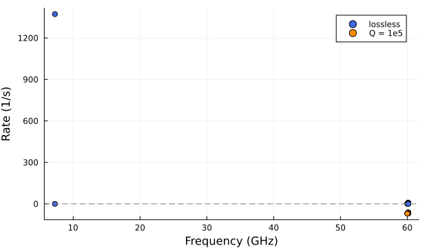

Locate the growing mode along the line

Use the same mode's voltage profile at the bus and resonator nodes to see where it is concentrated. Resolve nodes through component names, so the plot does not depend on the compiled node ordering:

compiled = compile(line)
cells = 1:256
resonators = [compiled.componentnamedict["cell$i/cr"] for i in cells]
junctions = [compiled.componentnamedict["cell$i/jj"] for i in cells]
profileaxis = Dict(name => i for (i, name) in enumerate(p.nodes))
resonatornodes = [profileaxis[compiled.nodenames[compiled.nodeindices[1, c]]] for c in resonators]
busnodes = [profileaxis[compiled.nodenames[compiled.nodeindices[1, c]]] for c in junctions]
k = 1  # the growing mode identified above
vr = sqrt.(vec(sum(abs2, p.nodevoltage[:, resonatornodes, k]; dims = 1)))
vb = sqrt.(vec(sum(abs2, p.nodevoltage[:, busnodes, k]; dims = 1)))
peak = max(maximum(vr), maximum(vb))
@assert peak > 0 && all(isfinite, vr) && all(isfinite, vb)
profile = plot(cells, hcat(vb, vr) ./ peak;
    label = ["Bus" "Resonator"], xlabel = "Cell",
    ylabel = "Relative voltage profile", size = (620, 360))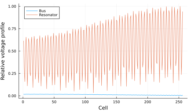

Each point is the square root of the sum of squared Fourier coefficients at that node. This measures the spatial amplitude of the periodic profile, independent of the arbitrary global eigenvector phase. Both traces use the same peak normalization. The plot shows relative voltage, not stored energy or a prediction of the eventual oscillation amplitude. Increase the profile window if its omitted harmonics matter, and refine steps independently to check the mode itself.

Reading a mode

A pole s and its coefficients q_n describe the perturbation

growing at the rate real(s), its coefficient n at the angular frequency imag(s) + n*Ω; a real perturbation is a mode and its conjugate. nodevoltage[i, node, pole] and junctionflux[i, junction, pole] hold the voltage and flux coefficients, normalized together, with modes[i] == (n,); modes lists the harmonics in the order of the discrete Fourier transform, 0 to H and then -H to -1. Eigenvector amplitude and global phase are arbitrary. The stored convention normalizes the combined squared norm of nodevoltage/frequencyscale and junctionflux to one for a nonzero exported profile. These are relative mode shapes, not absolute driven voltages or fluxes.

Each pole has Floquet aliases, s + im*k*Ω. The period map returns one representative of each selected mode, normally placed at its dominant physical harmonic, n = 0. Its time sampling must resolve that harmonic; increasing only the profile window cannot repair a frequency aliased by the time step. The polynomial methods truncate the harmonics and can return several approximate aliases of a physical mode: a search returns whichever lie nearest its shift, and on a long pumped line most poles near a band are aliases of modes far above it. harmonics gives each mode's dominant harmonic n: the mode lives mostly at imag(s) + n*Ω, which tells the aliases apart by their content. A mode whose dominant harmonic is an outermost one, or whose edgeweights are large needs a wider harmonic window. This changes the polynomial eigenproblem, but only the exported profile for Monodromy. An internal mode may have a zero node/junction profile; see the limitations below before interpreting its reported frequency.

Without nonlinear or pumpfrequency the analysis is unpumped, with the one harmonic 0, and the default finds every pole of its polynomial; a negative resistor checks the sign, growing at -1/(R*C):

using JosephsonCircuits
rlc = hbstability(Circuit([(:r, 1, 0, Resistor(2.0)),
    (:c, 1, 0, Capacitor(0.5)), (:l, 1, 0, Inductor(2.0))]))
@assert all(isapprox.(real.(rlc.poles), -0.5))
@assert sort(imag.(rlc.poles)) ≈ [-sqrt(3)/2, sqrt(3)/2]
active = hbstability(Circuit([(:r, 1, 0, Resistor(-2.0)), (:c, 1, 0, Capacitor(0.5))]))
@assert only(active.poles) ≈ 1.0
(rlc.poles, active.poles)

(ComplexF64[-0.49999999999999983 + 0.8660254037844385im, -0.5000000000000001 - 0.8660254037844387im], ComplexF64[0.9999999999999998 + 0.0im])

Delays and Laplace models

An exact TransmissionLine delay or a LaplaceResponse model makes the operator transcendental, and ContourIntegral finds its poles inside a circle. The period map of a pumped circuit takes a line's delay in time instead, its history over the delay part of the map's state; a LaplaceResponse model, which has no realization in time, and the delays of an unpumped circuit need the contour. A line between two mismatched resistors has the ladder s = (-log(2) + im*k*pi)/tau, three of which this circle holds:

using JosephsonCircuits
line = Circuit([
    (:left, 1, 0, Resistor(150.0)),
    (:right, 2, 0, Resistor(150.0)),
    (:line, 1, 2, TransmissionLine(50.0, 0.02; vp = 2e8)),
])
p = hbstability(line; method = ContourIntegral(-log(2)/1e-10, 4/1e-10),
    frequencyscale = 1e10)
expected = [(-log(2) + im*k*pi)/1e-10 for k in -1:1]
@assert p.converged && length(p.poles) == 3
@assert maximum(minimum(abs.(s .- expected)) for s in p.poles) < 1e-6/1e-10
p.poles

3-element Vector{ComplexF64}:
 -6.931471805599453e9 + 3.141592653589795e10im
 -6.931471805599459e9 - 8.8108933174919e-7im
 -6.931471805599461e9 - 3.141592653589794e10im

A LaplaceResponse states a component's analytic continuation, which harmonic balance evaluates at s = im*w:

using JosephsonCircuits
f = LaplaceResponse(s -> 50*(1 + s/1e10))
r = Resistor(FrequencyDependent(f))
block = ScatteringParameters(LaplaceResponse(s -> fill(0.2/(1 + s/1e10), 1, 1));
    nports = 1, zref = 50.0)
@assert f(1e10) == 50 + 50im

A table or a callable of real frequency has no continuation: fit it with RationalScattering, whose states the poles keep, and solve the operating point with the fit.

Interpreting accuracy

There are three separate questions:

1. Was the finite eigenproblem solved? converged, residuals, and searches describe numerical acceptance and search convergence. For a polynomial method, residuals is a relative backward error. For pumped Monodromy it is a condition-based estimate of multiplier roundoff, relative to the multiplier. It excludes time-discretization error.

2. Does the discretization represent the operating point and its modes? Increase the pump harmonics and either the perturbation harmonics or Monodromy's steps. Match modes when comparing solves. Modes far above the pump and weak growth/decay rates often need the most refinement.

3. Did the search cover the modes relevant to stability? A local shift or contour can miss an instability elsewhere. Monodromy computes all multipliers of its finite map, then returns at most nev resolved modes. DenseSpectrum examines the full finite pencil. Neither makes the underlying continuous problem complete at an insufficient discretization.

For pumped Monodromy, let M_N and M_2N be the coarse and refined maps. Line histories are resampled for the refined propagation and read back in the coarse coordinates. With V and U the selected modes' right and left vectors, the estimate projects the refined map onto them,

where μ_2N is the eigenvalue of G whose eigenvector carries most of the coarse mode, and 16/15 scales the change to the coarse map's error at the Gauss–Legendre rule's fourth order. G follows the mixing among the selected modes; mixing with modes beyond nev is not followed. The implementation returns Inf when no eigenvector of G carries more than half of the mode. A map too coarse for its error to fall as the fourth power of the step can have more error than its estimate.

abs(real(s)) > rateerrors[k] is evidence of a resolved sign, growth where real(s) > rateerrors[k] and decay where real(s) < -rateerrors[k], not a certificate. Near a stability boundary, repeat the full analysis with more steps until matched rates and their signs settle and the estimate falls about sixteenfold as the steps double. Where modes crowd, also check the result's sensitivity to nev: timestep refinement alone does not test the coupling to omitted modes. Cross-check another method when practical.

Gauss–Legendre stepping is not L-stable. A decay much faster than one step can appear as a slowly decaying discrete mode. Resolve the circuit's fast decays as well as its high oscillation frequencies; a small reported rateerrors alone is insufficient. Transmission-line history interpolation also contributes discretization error.

An unstable pole indicates growth of an infinitesimal perturbation of the chosen operating point. It does not predict the final nonlinear state or its amplitude. A transientsolve calculation started near that orbit with a perturbation that overlaps the mode can provide an independent check of early-time growth. Failure to see growth during a finite run does not establish stability if the seed is too small or the mode grows slowly.

Supported models and troubleshooting

Use the same circuit, component definitions, and terminations as the HB solve. Independent drives are held fixed when perturbing the orbit. Startup envelopes of pumped scattering blocks are ignored: stability is evaluated with their conversion fully on, as in harmonic balance.

Model	Applicable methods
Constant real lumped elements, junctions/nonlinear inductors, mutual inductors, constant or rational scattering blocks	Polynomial methods; pumped Monodromy when the model has a supported time-domain realization
Exact TransmissionLine	Pumped Monodromy or ContourIntegral; unpumped analysis requires ContourIntegral
LaplaceResponse or analytic conversion harmonics	ContourIntegral; a purely frequency-domain analytic response has no transient realization
Tabulated scattering data or a callable of real frequency	First supply a causal rational fit or analytic Laplace model, and recompute the HB operating point with that model

For pumped Monodromy each line's delay must be at least one timestep: T/steps <= minimum_delay. Also require 2H + 1 <= steps for the exported profile window. More steps increase both the propagation work and the number of line-history coordinates.

Observation	Next step
converged == false	Inspect the method's search diagnostics and rejected candidates; refine the search before interpreting its coverage
rateerrors[k] == Inf	Double steps and compare full solves; match profiles rather than assuming the same array index
A small positive or negative rate	Refine the operating point and discretization; compare rate changes against the rate, not the oscillation frequency
Large edgeweights	Increase H; with Monodromy this widens the profile only, so refine steps separately
Zero profiles or internalonly[k]	The mode may be internal to a block or line. It is not necessarily absent or harmless, and profile matching cannot follow it
Orbit initialization or algebraic consistency fails	Check HB convergence, circuit/definition identity, source reconstruction, and a supported transient realization; do not simply loosen the check to admit a different orbit
The recorded orbit does not close accurately over a period	Refine HB harmonics and time steps and check the model/drive agreement before treating its map as a Floquet map
A GPU eigensolver is unavailable	Use Monodromy() with its default CPU backend; the device path requires a CUDA runtime with cuSOLVER 11.7.1 or newer, which CUDA.jl checks at the eigensolve

A mode hidden in a transmission line, with no node/junction or rational-state content, is placed by the waves leaving the line's ports; its exported profile is zero.

How the period map works

Let δx contain the circuit's constrained perturbations: node fluxes and rates, rational-block states, and sampled outgoing-wave histories for transmission lines. Algebraic constraints determine auxiliary currents and constrain admissible starts; unobservable uniform-flux gauge directions are removed. These are circuit state/history coordinates, not an S-parameter matrix or a basis of input/output port waves.

The tangent dynamics along one recorded HB orbit define

A multiplier's magnitude gives growth (abs(μ) > 1) or decay (abs(μ) < 1) in the discrete map. The logarithm leaves the imaginary part ambiguous by integer multiples of Ω. Propagating a selected eigenvector through the period and Fourier analyzing its periodic part normally picks the representative at its dominant physical harmonic and supplies its profile. The number of returned representatives is limited by nev.

The implementation forms a dense map and calls a dense eigensolver. On CPU it balances the map, computes its real Schur form and all multipliers, then forms only the selected left/right eigenvectors. With Monodromy(backend=CUDABackend()), load CUDA.jl and CUDSS.jl; propagation and the dense eigensolve use the device, while balancing, selection, and constraint setup remain on the host. The device solver computes all right eigenvectors and obtains selected left vectors from their basis, each checked against its residual; where the basis is singular or ill-conditioned, the CPU's Schur path solves the map instead.

For map dimension d, storage grows as O(d^2) and the dense eigensolve as O(d^3). Reducing nev reduces selected-vector and profile work, but not the full map or eigenvalue calculation. A line of delay τ adds about 2τ/dt history coordinates, so timestep refinement can also increase d. For a large circuit, use a local polynomial or contour search when a restricted spectral region answers the question, while recognizing its limited coverage.

The orbit is recorded with transientsolve and its tangent is propagated with transienttangent. Initial block states and line histories are reconstructed from the HB orbit. This shares the circuit dynamics with transient analysis, but does not remove discretization or orbit-reconstruction error.

What enters the polynomial

The variational equation of a lumped circuit, C δΦ'' + G δΦ' + K(t) δΦ = 0, with the junctions' stiffness along the orbit in K(t), becomes in the harmonics

the operator hblinsolve solves at s = im*w, from the same modulation. Floating node fluxes are replaced by their voltages, so that a capacitor with no path to ground keeps its zero pole and an RC network its decay. Ports keep their terminations and sources perturb nothing; scattering blocks keep their port currents and their internal states, a pumped block its conversions with its pump phase. The polynomial in λ = s/frequencyscale, its rows equilibrated, has the companion pencil

which DenseSpectrum solves densely and ShiftInvert inverts at a shift σ without forming it, a = -Q(σ)^{-1}[(Q_1 + σQ_2)u + Q_2 v] and b = u + σa for the input [u; v], one factorization of Q(σ) a shift. ContourIntegral reduces the moments of Q(s)^{-1} around its circle (Beyn, Linear Algebra Appl. 436, 2012). Every pole is accepted on its backward error in Q, ‖Q(λ)q‖/((max‖Q_j‖ + |λ|‖Q_1‖ + |λ|²‖Q_2‖)‖q‖).