SNAIL Parametric Amplifier

Compare pump-on and pump-off gain for an explicitly modeled SNAIL. The quadratic nonlinearity supports three-wave mixing. Similar resonance frequencies in the two curves indicate operation near the chosen Kerr-free point.

Requires JosephsonCircuits and Plots. The optional comparison uses WRspice through XicTools_jll, or a local WRspice installation.

The SNAIL follows Frattini et al. (2018). A resonator, lr and cr, ends in a SNAIL: a small junction jj1 in a loop with three large ones in series, jj2 to jj4, and the loop inductance ll; port 2, of 1 kΩ, drives the bias line ldc, coupled to ll by k1. The small junction has alpha times the area of the large ones, so alpha times their critical current and capacitance. The resonator, 1.25 times that of the flux-pumped example, and the bias line, Ll, Ldc and K of that example, are assumed, as are the bias and the pump, at twice the pump-off resonance of 8.019 GHz:

text

 1          2          3             4                5                6
 o---[cc]---o---[lr]---o----[ll]-----o--[jj2 || cj2]--o--[jj3 || cj3]--o
 |          |          |                                               |
[p1]      [cr]   [jj1 || cj1]                                    [jj4 || cj4]
 |          |          |                                               |
 o----------o----------o-----------------------------------------------o
 0

 7
 o
 |
[p2 || ldc]      ldc coupled to ll by k1
 |
 o
 0

julia

using JosephsonCircuits
using Plots

R = 50.0
Cc = 0.048e-12
Cj = 10.0e-15
Lj = 60e-12
Cr = 0.4e-12*1.25
Lr = 0.4264e-9*1.25
Ll = 34e-12
Ldc = 0.74e-12
K = 0.999 # the coupling of the bias inductor ldc to the loop inductor ll

alpha = 0.29 # the area of the small junction relative to the large ones
circuit = Circuit(
    [(:p1, 1, 0, Port(1; Z0 = R)),
     (:cc, 1, 2, Capacitor(Cc)),
     (:lr, 2, 3, Inductor(Lr)), (:cr, 2, 0, Capacitor(Cr)),
     # the small junction of the SNAIL, across the three large ones
     (:jj1, 3, 0, JosephsonJunction(Lj/alpha)),
     (:cj1, 3, 0, Capacitor(alpha*Cj)),
     (:ll, 3, 4, Inductor(Ll)),
     (:jj2, 4, 5, JosephsonJunction(Lj)), (:cj2, 4, 5, Capacitor(Cj)),
     (:jj3, 5, 6, JosephsonJunction(Lj)), (:cj3, 5, 6, Capacitor(Cj)),
     (:jj4, 6, 0, JosephsonJunction(Lj)), (:cj4, 6, 0, Capacitor(Cj)),
     # the bias inductor, mutually coupled to the loop inductor ll
     (:ldc, 7, 0, Inductor(Ldc)),
     (:k1, :ll, :ldc, MutualInductor(K)),
     # a high impedance port, so the bias may be applied across it
     (:p2, 7, 0, Port(2; Z0 = 1000.0))])
ws = 2*pi*(7.8:0.001:8.2)*1e9
wp = (2*pi*16.038*1e9,)
Ip = 4.7e-6
Idc = 0.000159
# add the DC bias and pump to port 2
sourcespumpon = [(mode=(0,),port=2,current=Idc),(mode=(1,),port=2,current=Ip)]
sourcespumpoff = [(mode=(0,),port=2,current=Idc),(mode=(1,),port=2,current=0.0)]
Npumpharmonics = (16,)
Nmodulationharmonics = (8,)

The full sweep and plotting commands continue this setup:

julia

jpapumpon = hbsolve(ws, wp, sourcespumpon, Nmodulationharmonics,
    Npumpharmonics, circuit, dc = true, threewavemixing=true,fourwavemixing=true) # enable dc and three wave mixing
@assert jpapumpon.nonlinear.solverinfo.converged
jpapumpoff = hbsolve(ws, wp, sourcespumpoff, Nmodulationharmonics,
    Npumpharmonics, circuit, dc = true, threewavemixing=true,fourwavemixing=true) # enable dc and three wave mixing
@assert jpapumpoff.nonlinear.solverinfo.converged

p1 = plot(
    jpapumpon.linearized.w/(2*pi*1e9),
    10*log10.(abs2.(
        jpapumpon.linearized.S(
            outputmode=(0,),
            outputport=1,
            inputmode=(0,),
            inputport=1,
            freqindex=:
        ),
    )),
    xlabel="Frequency (GHz)",
    ylabel="Gain (dB)",
    label="pump on",
)

plot!(
    jpapumpoff.linearized.w/(2*pi*1e9),
    10*log10.(abs2.(
        jpapumpoff.linearized.S(
            outputmode=(0,),
            outputport=1,
            inputmode=(0,),
            inputport=1,
            freqindex=:
        ),
    )),
    label="pump off",
)

p2 = plot(
    jpapumpon.linearized.w/(2*pi*1e9),
    angle.(
        jpapumpon.linearized.S(
            outputmode=(0,),
            outputport=1,
            inputmode=(0,),
            inputport=1,
            freqindex=:
        ),
    ),
    xlabel="Frequency (GHz)",
    ylabel="Phase (rad)",
    label="pump on",
)

plot!(
    jpapumpoff.linearized.w/(2*pi*1e9),
    angle.(
        jpapumpoff.linearized.S(
            outputmode=(0,),
            outputport=1,
            inputmode=(0,),
            inputport=1,
            freqindex=:
        ),
    ),
    label="pump off",
)
plot(p1,p2,layout=(2,1))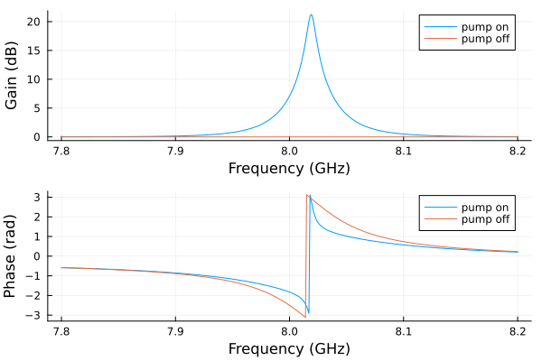

A small executable check

The documentation build uses the same circuit and bias/pump sources at three signal frequencies. The smaller harmonic limits check the workflow; refine them for a quantitative gain prediction.

julia

small = hbsolve(2pi .* [7.9e9, 8.0e9, 8.1e9], wp, sourcespumpon,
    (4,), (8,), circuit; dc = true, threewavemixing = true,
    fourwavemixing = true, atol = 1e-8)
@assert small.nonlinear.solverinfo.converged
@assert all(isfinite, small.linearized.S)
@assert maximum(abs.(abs.(small.linearized.CM) .- 1)) < 1e-5

With the pump and the bias off the circuit is linear, and its reflection has a closed form: the junctions are their inductances at zero phase, and the loop of the bias line, ldc and the 1 kΩ port, is reflected into ll through the mutual inductance M = K sqrt(Ll Ldc):

julia

function reflection(w)
    M = K*sqrt(Ll*Ldc)
    Zll = im*w*Ll + (w*M)^2/(im*w*Ldc + 1000.0)
    ZJ = 1/(1/(im*w*Lj) + im*w*Cj)
    Zsnail = 1/(1/(im*w*Lj/alpha) + im*w*alpha*Cj + 1/(Zll + 3ZJ))
    Z = 1/(im*w*Cc) + 1/(im*w*Cr + 1/(im*w*Lr + Zsnail))
    return (Z - R)/(Z + R)
end
wcheck = 2pi .* [7.9e9, 8.0e9, 8.1e9]
S11 = hblinsolve(wcheck, circuit).S((0,), 1, (0,), 1, :)
@assert isapprox(S11, reflection.(wcheck); atol = 1e-12)
(solver = S11, closed = reflection.(wcheck))

(solver = ComplexF64[0.9343393204281113 - 0.3563834643863663im, 0.9223075802703117 - 0.3864549853736003im, 0.9033349735133428 - 0.4289334464887074im], closed = ComplexF64[0.9343393204281112 - 0.35638346438636637im, 0.9223075802703119 - 0.3864549853736004im, 0.903334973513343 - 0.4289334464887074im])

Compare with WRspice

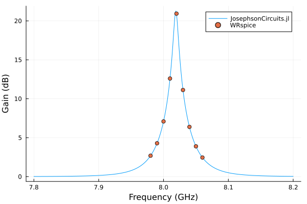
WRspice solves two 600 ns transients at each signal frequency, so the comparison is made at nine frequencies around the gain peak:

julia

using XicTools_jll

# simulate the SNAIL amplifier in WRSPICE
wswrspice=2*pi*(7.98:0.01:8.06)*1e9
n = JosephsonCircuits.exportnetlist(circuit);
input = JosephsonCircuits.wrspice_input_paramp(n.netlist,wswrspice,[0.0,wp[1]],[Idc,2*Ip],[(0,1)],[(0,7),(0,7)];trise=10e-9,tstop=600e-9);

output = JosephsonCircuits.spice_run(input,XicTools_jll.wrspice());
S11,S21=JosephsonCircuits.wrspice_calcS_paramp(output,wswrspice,n.Nnodes);

# plot the output
plot(
    jpapumpon.linearized.w/(2*pi*1e9),
    10*log10.(abs2.(
        jpapumpon.linearized.S(
            outputmode=(0,),
            outputport=1,
            inputmode=(0,),
            inputport=1,
            freqindex=:
        ),
    )),
    xlabel="Frequency (GHz)",
    ylabel="Gain (dB)",
    label="JosephsonCircuits.jl",
)

plot!(wswrspice/(2*pi*1e9),10*log10.(abs2.(S11)),
    label="WRspice",
    seriestype=:scatter)

SNAIL Parametric Amplifier ​

A small executable check ​

Compare with WRspice ​

SNAIL Parametric Amplifier

A small executable check

Compare with WRspice