Pumped finite-window gain and noise

This one-port Josephson amplifier starts at passive equilibrium, ramps its pump, and measures a weak finite-duration signal near 4.6 GHz. The input and output windows differ, so the reported gain includes the response to the probe's edges and the circuit's memory. Requires JosephsonCircuits and Plots.

 1
 o--------+--------+
 |        |        |
[p1]    [jj]     [cj]
 |        |        |
 o--------+--------+
 0

The calculation propagates Gaussian fluctuations about a nonlinear classical trajectory. It does not simulate a full nonlinear quantum state. Read the quantum-noise guide for normalization and the distinction between internal added noise and total output covariance.

Ramp from equilibrium

The 50 Ω port loads a parallel junction and capacitor, a resonance near 5 GHz of quality factor 50*sqrt(C/Lj), about 16. The pump is zero before the record starts and has a smooth 4 ns turn-on. Its 200 nA current is a peak time-domain amplitude, not an HB Fourier coefficient.

using JosephsonCircuits, LinearAlgebra, Plots
circuit = Circuit([
    (:p1, 1, 0, Port(1; Z0 = 50.0)),
    (:jj, 1, 0, JosephsonJunction(100e-12)),
    (:cj, 1, 0, Capacitor(10e-12)),
])
wp, ws = 2pi*4.75e9, 2pi*4.6e9
rise(t) = t <= 0 ? 0.0 : t >= 4e-9 ? 1.0 : sinpi(t/8e-9)^2
pump(wp) = t -> 200e-9*rise(t)*cos(wp*t)
problem = transientproblem(circuit; sources = [TransientSource(1, pump(wp))])
T = 24e-9
function trajectory(dt)
    # N samples cover the half-open Fourier record [0,T).
    transientsolve(problem, (0.0, T - dt); dt,
        method = GaussLegendre(), record = :phases)
end
solution = trajectory(5e-12)
@assert all(isfinite, solution.voltage)

Recording phases makes the trajectory available to tangent and adjoint calculations. The initial mean state is zero, but initial quantum fluctuations are not: transientnoise initializes each bath's stationary response about that passive equilibrium. Starting the record after an already-running pump would violate this initial-noise assumption.

Define input and output modes

Each window has a smooth sine-squared envelope. The mode constructor projects the carrier/envelope onto positive Fourier bins and normalizes it; photon normalization includes the frequency of each bin. The output window extends four nanoseconds beyond the input window.

function windowplan(sol, a, b)
    times = sol.times[round(Int, a/sol.dt) + 1:round(Int, b/sol.dt)]
    envelope = reshape(sinpi.((times .- a)./(b - a)).^2, :, 1)
    transientquantumplan(sol, times, [ws]; ports = [1], envelopes = envelope)
end
input = windowplan(solution, 8e-9, 16e-9)
output = windowplan(solution, 8e-9, 20e-9)
G = transientgain(solution, output, input)
@assert minimum(svdvals(G)) > 1
G

2×2 Matrix{Float64}:
 1.96883   -0.380216
 0.383016   2.00712

G maps the input's (X,P) to the measured output's (X,P) for a probe applied only inside the input window. Its singular values are quadrature amplitude gains; their squares are the extremal photon gains for input quadrature directions. They are about 2 in amplitude in this example. They need not equal a monochromatic HB gain.

times = solution.times
envelope(t, a, b) = a <= t <= b ? sinpi((t - a)/(b - a))^2 : 0.0
p = plot(times .* 1e9, rise.(times); label = "pump ramp", color = :black,
    xlabel = "Time (ns)", ylabel = "Envelope (arbitrary scale)")
plot!(p, times .* 1e9, envelope.(times, 8e-9, 16e-9); label = "input window")
plot!(p, times .* 1e9, envelope.(times, 8e-9, 20e-9); label = "output window")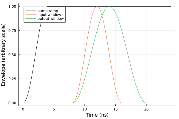

Total output covariance

Use a bath band broad enough to include pump-converted noise, not only the signal bin. Here the first pass uses all positive record bins up to 20 GHz, a cutoff of 2pi*20e9 rad/s, with spacing and weight 2pi/T. The port termination is the only bath and is at zero temperature.

noise = transientnoise(solution, output; cutoff = 2pi*20e9)
@assert noise.diagnostics.passed
@assert isapprox(noise.addedcovariance, zeros(2,2); atol = 1e-12)
(noise.covariance, noise.diagnostics)

([4.677142285216192 -0.38922832215553577; -0.38922832215553577 4.72317369146926], (commutationerror = 3.97105864968772e-6, minimumuncertaintyeigenvalue = 4.066100885742004, passed = true))

The full output covariance is about [4.68 -0.39; -0.39 4.72] in quanta, compared with vacuum I/2. It includes fluctuations entering from every bath mode that mixes into this output. There are no internal dissipative baths, so addedcovariance is zero even though the total noise is amplified. addedcovariance therefore differs from the added noise referred to a selected signal mode in amplifier theory.

The optional inputs gain in transientnoise requires input and output plans on exactly the same window and drives periodically extended modes with stationary prehistory. The distinct windows here belong in transientgain. Its causal gain and the total output covariance characterize this particular finite-window measurement. The covariance has unequal principal variances, so retain the matrix description. A scalar transientquantumefficiency requires the appropriate phase-insensitive gain/noise conditions; it is not an automatic summary of every pulsed experiment.

Refine three independent choices

First halve the timestep at the same physical windows and bath cutoff. Then raise the cutoff while keeping that trajectory fixed. Finally halve the frequency spacing with an explicit quadrature, keeping cutoff, step, and windows fixed. This last check changes the approximation to the continuous bath without changing the classical record.

fine = trajectory(2.5e-12)
fine_input = windowplan(fine, 8e-9, 16e-9)
fine_output = windowplan(fine, 8e-9, 20e-9)
fine_G = transientgain(fine, fine_output, fine_input)
step_noise = transientnoise(fine, fine_output; cutoff = 2pi*20e9)
cutoff_noise = transientnoise(fine, fine_output; cutoff = 2pi*30e9)
dw = pi/T   # half the record's bin spacing 2pi/T
bath_frequencies = collect(dw:dw:2pi*30e9)
grid_noise = transientnoise(fine, fine_output;
    frequencies = bath_frequencies, weights = fill(dw, length(bath_frequencies)))

relative_change(a, b) = norm(a - b)/norm(b)
changes = (
    gain_step = relative_change(G, fine_G),
    covariance_step = relative_change(noise.covariance, step_noise.covariance),
    covariance_cutoff = relative_change(step_noise.covariance, cutoff_noise.covariance),
    covariance_spacing = relative_change(cutoff_noise.covariance, grid_noise.covariance),
)
@assert all(r -> r.diagnostics.passed, (noise, step_noise, cutoff_noise, grid_noise))
@assert maximum(values(changes)) < 1e-3
changes

(gain_step = 3.123582246396336e-5, covariance_step = 0.00011374917848677393, covariance_cutoff = 5.075086159496027e-7, covariance_spacing = 5.732867079856595e-7)

For this example the gain changes by roughly 3e-5 and the covariance by 1e-4 on timestep refinement; the cutoff and spacing changes are smaller. These differences are empirical convergence evidence, not certified error bounds. A passed commutator/uncertainty check alone would not establish them. Near threshold, with sharper pulses, or with a higher-Q circuit, repeat the refinements until the observables meet your accuracy target.

Also vary the pump ramp/prehistory and window placement when asking whether the measurement represents a settled amplifier. Varying the measurement window changes the physical temporal mode, so a change in its gain or covariance need not be a numerical error. Refining a sampled window should keep its physical duration, envelope, carrier, and phase reference fixed, as done here. The adjacent ten-signal recipe shows how to construct a more complex classical drive before applying these steps.