Josephson parametric amplifier (JPA)

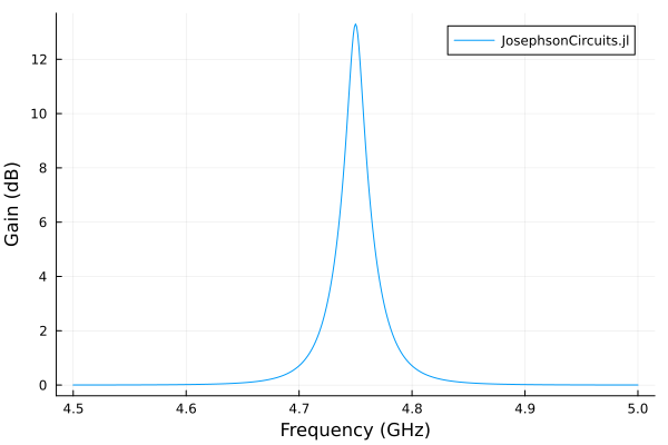
Calculate reflection gain near the resonance of a current-pumped JPA, then compare with WRspice. The signal-frequency sweep uses the small-signal response about the strong pump. Refine both harmonic limits before interpreting the peak gain.

Requires JosephsonCircuits and Plots. The optional comparison uses WRspice through XicTools_jll, or a local WRspice installation.

For temporal stability of this pumped circuit, continue with the worked pole-analysis example, including harmonic refinement.

A 50 Ω port couples through cc to a junction shunted by cj:

 1                  2
 o------[cc]--------o--------+
 |                  |        |
[p1]              [jj]     [cj]
 |                  |        |
 o------------------o--------+
 0

using JosephsonCircuits

R = 50.0
Cc = 100.0e-15
Lj = 1000.0e-12
Cj = 1000.0e-15

# each entry is the name, the nodes of the two terminals, and the
# component; node 0 is ground
circuit = Circuit(
    [(:p1, 1, 0, Port(1; Z0 = R)),
     (:cc, 1, 2, Capacitor(Cc)),
     (:jj, 2, 0, JosephsonJunction(Lj)),
     (:cj, 2, 0, Capacitor(Cj))])

ws = 2*pi*(4.5:0.001:5.0)*1e9
wp = (2*pi*4.75001*1e9,)
Ip = 0.00565e-6
sources = [(mode=(1,),port=1,current=Ip)]
Npumpharmonics = (16,)
Nmodulationharmonics = (8,)

The sweep and its plot:

using Plots
jpa = hbsolve(ws, wp, sources, Nmodulationharmonics,
    Npumpharmonics, circuit)
@assert jpa.nonlinear.solverinfo.converged

plot(
    jpa.linearized.w/(2*pi*1e9),
    10*log10.(abs2.(
        jpa.linearized.S(
            outputmode=(0,),
            outputport=1,
            inputmode=(0,),
            inputport=1,
            freqindex=:
        ),
    )),
    label="JosephsonCircuits.jl",
    xlabel="Frequency (GHz)",
    ylabel="Gain (dB)",
)

Compare with WRspice. Please note that on Linux you can install the XicTools_jll package which provides WRspice for x86_64. For other operating systems and platforms, you can install WRspice yourself and substitute XicTools_jll.wrspice()withJosephsonCircuits.wrspice_cmd() which will attempt to provide the path to your WRspice executable.

using XicTools_jll

wswrspice=2*pi*(4.5:0.01:5.0)*1e9
n = JosephsonCircuits.exportnetlist(circuit);
input = JosephsonCircuits.wrspice_input_paramp(n.netlist,wswrspice,wp[1],2*Ip,(0,1),(0,1));

output = JosephsonCircuits.spice_run(input,XicTools_jll.wrspice());
S11,S21=JosephsonCircuits.wrspice_calcS_paramp(output,wswrspice,n.Nnodes);

plot!(wswrspice/(2*pi*1e9),10*log10.(abs2.(S11)),
    label="WRspice",
    seriestype=:scatter)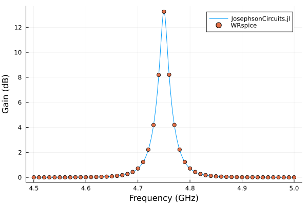

A small executable check

The documentation build solves the same circuit and pump at three signal frequencies, the middle one the peak of the gain:

small = hbsolve(2pi .* [4.6e9, 4.75e9, 4.9e9], wp, sources,
    Nmodulationharmonics, Npumpharmonics, circuit)
@assert small.nonlinear.solverinfo.converged
@assert maximum(abs.(abs.(small.linearized.CM) .- 1)) < 1e-8
round.(10 .* log10.(abs2.(small.linearized.S((0,), 1, (0,), 1, :))); digits = 2)

1-dimensional KeyedArray(NamedDimsArray(...)) with keys:
↓   freqindex ∈ 3-element UnitRange{Int64}
And data, 3-element Vector{Float64}:
 (1)   0.02
 (2)  13.3
 (3)   0.02