Examples

Josephson parametric amplifier (JPA)

A driven nonlinear LC resonator.

using JosephsonCircuits
using Plots

R = 50.0
Cc = 100.0e-15
Lj = 1000.0e-12
Cj = 1000.0e-15

# each entry is the name, the nodes of the two terminals, and the
# component; node 0 is ground
circuit = Circuit(
    [(:p1, 1, 0, Port(1; Z0 = R)),
     (:cc, 1, 2, Capacitor(Cc)),
     (:jj, 2, 0, JosephsonJunction(Lj)),
     (:cj, 2, 0, Capacitor(Cj))])

ws = 2*pi*(4.5:0.001:5.0)*1e9
wp = (2*pi*4.75001*1e9,)
Ip = 0.00565e-6
sources = [(mode=(1,),port=1,current=Ip)]
Npumpharmonics = (16,)
Nmodulationharmonics = (8,)

@time jpa = hbsolve(ws, wp, sources, Nmodulationharmonics,
    Npumpharmonics, circuit)

plot(
    jpa.linearized.w/(2*pi*1e9),
    10*log10.(abs2.(
        jpa.linearized.S(
            outputmode=(0,),
            outputport=1,
            inputmode=(0,),
            inputport=1,
            freqindex=:
        ),
    )),
    label="JosephsonCircuits.jl",
    xlabel="Frequency (GHz)",
    ylabel="Gain (dB)",
)

  0.001817 seconds (12.99 k allocations: 4.361 MiB)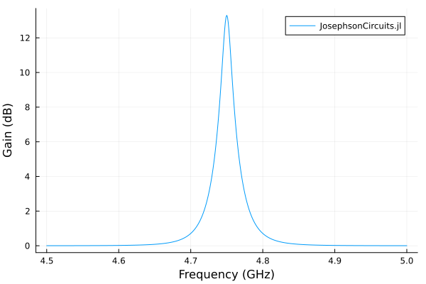

Compare with WRspice. Please note that on Linux you can install the XicTools_jll package which provides WRspice for x86_64. For other operating systems and platforms, you can install WRspice yourself and substitute XicTools_jll.wrspice()withJosephsonCircuits.wrspice_cmd() which will attempt to provide the path to your WRspice executable.

using XicTools_jll

wswrspice=2*pi*(4.5:0.01:5.0)*1e9
n = JosephsonCircuits.exportnetlist(circuit);
input = JosephsonCircuits.wrspice_input_paramp(n.netlist,wswrspice,wp[1],2*Ip,(0,1),(0,1));

@time output = JosephsonCircuits.spice_run(input,XicTools_jll.wrspice());
S11,S21=JosephsonCircuits.wrspice_calcS_paramp(output,wswrspice,n.Nnodes);

plot!(wswrspice/(2*pi*1e9),10*log10.(abs2.(S11)),
    label="WRspice",
    seriestype=:scatter)

 12.743245 seconds (32.66 k allocations: 499.263 MiB, 0.41% gc time)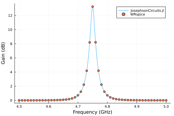

JPA with a frequency dependent environmental impedance

Any component value can be a function of frequency: FrequencyDependent wraps an arbitrary Julia closure of the signed mode frequency in radians per second, and both the nonlinear pump solve and the linearized sweep evaluate it at their own mode frequencies. Here the JPA of the first example sees its environment through five centimeters of slightly mismatched cable – a 50 ohm line terminated by a 40 ohm source – so the port resistor becomes the complex input impedance of that line. The transformed environment reshapes the gain and moves the peak, and because the pump harmonics feel it too, the operating point itself shifts, not just the readout. A physical impedance obeys Z(-w) = conj(Z(w)), which this law satisfies automatically because tan is odd and the constants are real.

using JosephsonCircuits
using Plots

Cc = 100.0e-15
Lj = 1000.0e-12
Cj = 1000.0e-15

# the input impedance of a mismatched cable between source and amplifier
Z0 = 50.0    # cable characteristic impedance, ohms
ZL = 40.0    # source impedance, ohms
len = 0.05   # cable length, meters
vp = 2.0e8   # cable phase velocity, meters per second
Zenv(w) = Z0*(ZL + im*Z0*tan(w*len/vp))/(Z0 + im*ZL*tan(w*len/vp))

amplifier(Zr) = Circuit(
    [(:p1, 1, 0, Port(1; Z0 = Zr)),
     (:cc, 1, 2, Capacitor(Cc)),
     (:jj, 2, 0, JosephsonJunction(Lj)),
     (:cj, 2, 0, Capacitor(Cj))])

ws = 2*pi*(4.5:0.001:5.0)*1e9
wp = (2*pi*4.75001*1e9,)
sources = [(mode=(1,), port=1, current=0.00565e-6)]

@time ideal = hbsolve(ws, wp, sources, (8,), (16,), amplifier(50.0))
@time cable = hbsolve(ws, wp, sources, (8,), (16,),
    amplifier(FrequencyDependent(Zenv)))

gain(sol) = 10*log10.(abs2.(sol.linearized.S(outputmode=(0,),
    outputport=1, inputmode=(0,), inputport=1, freqindex=:)))
plot(ws/(2*pi*1e9), [gain(ideal) gain(cable)],
    label=["ideal 50 ohm environment" "through mismatched cable"],
    xlabel="Frequency (GHz)", ylabel="Gain (dB)")

Double-pumped Josephson parametric amplifier (JPA)

using JosephsonCircuits
using Plots

R = 50.0
Cc = 100.0e-15
Lj = 1000.0e-12
Cj = 1000.0e-15

# each entry is the name, the nodes of the two terminals, and the
# component; node 0 is ground
circuit = Circuit(
    [(:p1, 1, 0, Port(1; Z0 = R)),
     (:cc, 1, 2, Capacitor(Cc)),
     (:jj, 2, 0, JosephsonJunction(Lj)),
     (:cj, 2, 0, Capacitor(Cj))])

ws = 2*pi*(4.5:0.001:5.0)*1e9
wp = (2*pi*4.65001*1e9,2*pi*4.85001*1e9)

Ip = 0.00565e-6*1.7
sources = [(mode=(1,0),port=1,current=Ip),(mode=(0,1),port=1,current=Ip)]
Npumpharmonics = (8,8)
Nmodulationharmonics = (8,8)

@time jpa = hbsolve(ws, wp, sources, Nmodulationharmonics,
    Npumpharmonics, circuit);

plot(
    jpa.linearized.w/(2*pi*1e9),
    10*log10.(abs2.(
        jpa.linearized.S(
            outputmode=(0,0),
            outputport=1,
            inputmode=(0,0),
            inputport=1,
            freqindex=:
        ),
    )),
    label="JosephsonCircuits.jl",
    xlabel="Frequency (GHz)",
    ylabel="S11 (dB)",
)

  0.182720 seconds (12.70 k allocations: 713.087 MiB)

and compare with WRspice

using XicTools_jll

wswrspice=2*pi*(4.5:0.01:5.0)*1e9
n = JosephsonCircuits.exportnetlist(circuit);
input = JosephsonCircuits.wrspice_input_paramp(n.netlist,wswrspice,[wp[1],wp[2]],[2*Ip,2*Ip],(0,1),[(0,1),(0,1)]);

@time output = JosephsonCircuits.spice_run(input,XicTools_jll.wrspice());
S11,S21=JosephsonCircuits.wrspice_calcS_paramp(output,wswrspice,n.Nnodes,stepsperperiod = 50000);

plot!(wswrspice/(2*pi*1e9),10*log10.(abs2.(S11)),
    label="WRspice",
    seriestype=:scatter)

 15.782862 seconds (32.80 k allocations: 509.192 MiB, 0.39% gc time)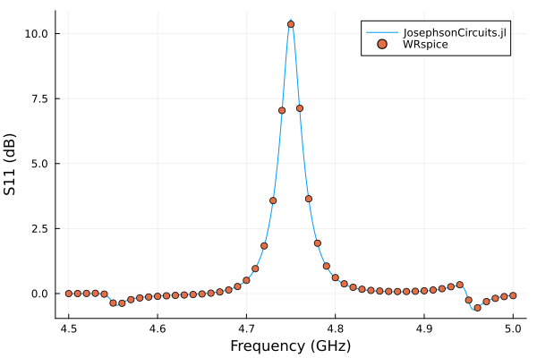

Flux-pumped Josephson parametric amplifier (JPA)

Circuit and parameters from here. Please note that three wave mixing (3WM) and flux-biasing are relatively untested, so you may encounter bugs. Please file issues or PRs.

using JosephsonCircuits
using Plots

R = 50.0
Cc = 16.0e-15
Cj = 10.0e-15
Lj = 219.63e-12
Cr = 0.4e-12
Lr = 0.4264e-9
Ll = 34e-12
Ldc = 0.74e-12
K = 0.999 # the inverse inductance matrix for K=1.0 diverges, so set K<1.0

circuit = Circuit(
    [(:p1, 1, 0, Port(1; Z0 = R)),
     (:cc, 1, 2, Capacitor(Cc)),
     (:lr, 2, 3, Inductor(Lr)), (:cr, 2, 0, Capacitor(Cr)),
     (:jj1, 3, 0, JosephsonJunction(Lj)), (:cj1, 3, 0, Capacitor(Cj)),
     (:ll, 3, 4, Inductor(Ll)),
     (:jj2, 4, 0, JosephsonJunction(Lj)), (:cj2, 4, 0, Capacitor(Cj)),
     # the bias inductor, mutually coupled to the loop inductor ll
     (:ldc, 5, 0, Inductor(Ldc)),
     (:k1, :ll, :ldc, MutualInductor(K)),
     # a high impedance port, so the bias may be applied across it
     (:p2, 5, 0, Port(2; Z0 = 1000.0))])

ws = 2*pi*(9.7:0.0001:9.8)*1e9
wp = (2*pi*19.50*1e9,)
Ip = 0.7e-6
Idc = 140.3e-6
# add the DC bias and pump to port 2
sourcespumpon = [(mode=(0,),port=2,current=Idc),(mode=(1,),port=2,current=Ip)]
Npumpharmonics = (16,)
Nmodulationharmonics = (8,)
@time jpapumpon = hbsolve(ws, wp, sourcespumpon, Nmodulationharmonics,
    Npumpharmonics, circuit, dc = true, threewavemixing=true,fourwavemixing=true) # enable dc and three wave mixing


plot(
    jpapumpon.linearized.w/(2*pi*1e9),
    10*log10.(abs2.(
        jpapumpon.linearized.S(
            outputmode=(0,),
            outputport=1,
            inputmode=(0,),
            inputport=1,
            freqindex=:
        ),
    )),
    xlabel="Frequency (GHz)",
    ylabel="Gain (dB)",
    label="JosephsonCircuits.jl",
)

  0.015623 seconds (22.07 k allocations: 80.082 MiB)

and compare with WRspice

using XicTools_jll

# simulate the JPA in WRSPICE
wswrspice=2*pi*(9.7:0.005:9.8)*1e9
n = JosephsonCircuits.exportnetlist(circuit);
input = JosephsonCircuits.wrspice_input_paramp(n.netlist,wswrspice,[0.0,wp[1]],[Idc,2*Ip],[(0,1)],[(0,5),(0,5)];trise=10e-9,tstop=600e-9);

# @time output = JosephsonCircuits.spice_run(input,JosephsonCircuits.wrspice_cmd());
@time output = JosephsonCircuits.spice_run(input,XicTools_jll.wrspice());
S11,S21=JosephsonCircuits.wrspice_calcS_paramp(output,wswrspice,n.Nnodes);

# plot the output
plot!(wswrspice/(2*pi*1e9),10*log10.(abs2.(S11)),
    label="WRspice",
    seriestype=:scatter)

283.557011 seconds (26.76 k allocations: 7.205 GiB, 0.66% gc time)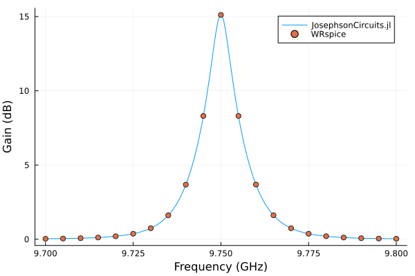

Simulate the JPA frequency as a function of DC bias current:

ws = 2*pi*(8.0:0.01:11.0)*1e9
currentvals = (-20:0.1:20)*1e-5
outvals = zeros(Complex{Float64},length(ws),length(currentvals))
Ip=0.0

Npumpharmonics = (1,)
Nmodulationharmonics = (1,)

@time for (k,Idc) in enumerate(currentvals)
    sources = [
          (mode=(0,),port=2,current=Idc),
          (mode=(1,),port=2,current=Ip),
      ]
    sol = hbsolve(ws,wp,sources,Nmodulationharmonics, Npumpharmonics,
        circuit;dc=true,threewavemixing=true,fourwavemixing=true)
    outvals[:,k]=sol.linearized.S((0,),1,(0,),1,:)
end

plot(
    currentvals/(1e-3),
    ws/(2*pi*1e9),
    10*log10.(abs2.(outvals)),
    seriestype=:heatmap,
    xlabel="bias current (mA)",
    ylabel="frequency (GHz)",
    title="S11 (dB), pump off",
)

0.219279 seconds (3.27 M allocations: 639.981 MiB, 20.84% gc time)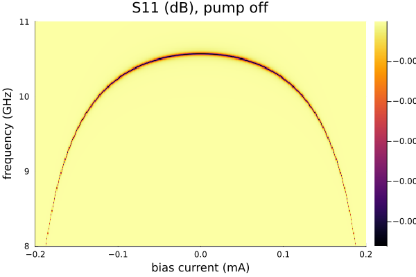

SNAIL Parametric Amplifier

Circuit parameters from here. Notice that the resonance frequency is similar for pump-on and pump-off, indicating it is operating near the Kerr-free point.

using JosephsonCircuits
using Plots

R = 50.0
Cc = 0.048e-12
Cj = 10.0e-15
Lj = 60e-12
Cr = 0.4e-12*1.25
Lr = 0.4264e-9*1.25
Ll = 34e-12
Ldc = 0.74e-12
K = 0.999 # the inverse inductance matrix for K=1.0 diverges, so set K<1.0

alpha = 0.29
Z0 = 50
w0 = 2*pi*8e9
l=10e-3
circuit = Circuit(
    [(:p1, 1, 0, Port(1; Z0 = R)),
     (:cc, 1, 2, Capacitor(Cc)),
     (:lr, 2, 3, Inductor(Lr)), (:cr, 2, 0, Capacitor(Cr)),
     # the small junction of the SNAIL, across the three large ones
     (:jj1, 3, 0, JosephsonJunction(Lj/alpha)),
     (:cj1, 3, 0, Capacitor(Cj/alpha)),
     (:ll, 3, 4, Inductor(Ll)),
     (:jj2, 4, 5, JosephsonJunction(Lj)), (:cj2, 4, 5, Capacitor(Cj)),
     (:jj3, 5, 6, JosephsonJunction(Lj)), (:cj3, 5, 6, Capacitor(Cj)),
     (:jj4, 6, 0, JosephsonJunction(Lj)), (:cj4, 6, 0, Capacitor(Cj)),
     # the bias inductor, mutually coupled to the loop inductor ll
     (:ldc, 7, 0, Inductor(Ldc)),
     (:k1, :ll, :ldc, MutualInductor(K)),
     # a high impedance port, so the bias may be applied across it
     (:p2, 7, 0, Port(2; Z0 = 1000.0))])

# ws = 2*pi*(9.7:0.0001:9.8)*1e9
# ws = 2*pi*(5.0:0.001:11)*1e9
ws = 2*pi*(7.8:0.001:8.2)*1e9
wp = (2*pi*16.00*1e9,)
Ip = 4.4e-6
# Idc = 140.3e-6
Idc = 0.000159
# add the DC bias and pump to port 2
sourcespumpon = [(mode=(0,),port=2,current=Idc),(mode=(1,),port=2,current=Ip)]
sourcespumpoff = [(mode=(0,),port=2,current=Idc),(mode=(1,),port=2,current=0.0)]
Npumpharmonics = (16,)
Nmodulationharmonics = (8,)
@time jpapumpon = hbsolve(ws, wp, sourcespumpon, Nmodulationharmonics,
    Npumpharmonics, circuit, dc = true, threewavemixing=true,fourwavemixing=true) # enable dc and three wave mixing
@time jpapumpoff = hbsolve(ws, wp, sourcespumpoff, Nmodulationharmonics,
    Npumpharmonics, circuit, dc = true, threewavemixing=true,fourwavemixing=true) # enable dc and three wave mixing

p1 = plot(
    jpapumpon.linearized.w/(2*pi*1e9),
    10*log10.(abs2.(
        jpapumpon.linearized.S(
            outputmode=(0,),
            outputport=1,
            inputmode=(0,),
            inputport=1,
            freqindex=:
        ),
    )),
    xlabel="Frequency (GHz)",
    ylabel="Gain (dB)",
    label="pump on",
)

plot!(
    jpapumpoff.linearized.w/(2*pi*1e9),
    10*log10.(abs2.(
        jpapumpoff.linearized.S(
            outputmode=(0,),
            outputport=1,
            inputmode=(0,),
            inputport=1,
            freqindex=:
        ),
    )),
    label="pump off",
)

p2 = plot(
    jpapumpon.linearized.w/(2*pi*1e9),
    angle.(
        jpapumpon.linearized.S(
            outputmode=(0,),
            outputport=1,
            inputmode=(0,),
            inputport=1,
            freqindex=:
        ),
    ),
    xlabel="Frequency (GHz)",
    ylabel="Gain (dB)",
    label="pump on",
)

plot!(
    jpapumpoff.linearized.w/(2*pi*1e9),
    angle.(
        jpapumpoff.linearized.S(
            outputmode=(0,),
            outputport=1,
            inputmode=(0,),
            inputport=1,
            freqindex=:
        ),
    ),
    label="pump off",
)
plot(p1,p2,layout=(2,1))

  0.010345 seconds (16.74 k allocations: 40.025 MiB)
  0.011252 seconds (16.68 k allocations: 39.985 MiB)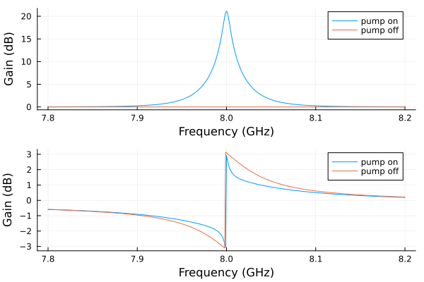

and compare with WRspice

using XicTools_jll

# simulate the JPA in WRSPICE
wswrspice=2*pi*(7.8:0.005:8.2)*1e9
n = JosephsonCircuits.exportnetlist(circuit);
input = JosephsonCircuits.wrspice_input_paramp(n.netlist,wswrspice,[0.0,wp[1]],[Idc,2*Ip],[(0,1)],[(0,7),(0,7)];trise=10e-9,tstop=600e-9);

@time output = JosephsonCircuits.spice_run(input,XicTools_jll.wrspice());
S11,S21=JosephsonCircuits.wrspice_calcS_paramp(output,wswrspice,n.Nnodes);

# plot the output
plot(
    jpapumpon.linearized.w/(2*pi*1e9),
    10*log10.(abs2.(
        jpapumpon.linearized.S(
            outputmode=(0,),
            outputport=1,
            inputmode=(0,),
            inputport=1,
            freqindex=:
        ),
    )),
    xlabel="Frequency (GHz)",
    ylabel="Gain (dB)",
    label="JosephsonCircuits.jl",
)

plot!(wswrspice/(2*pi*1e9),10*log10.(abs2.(S11)),
    label="WRspice",
    seriestype=:scatter)

2067.364975 seconds (149.73 k allocations: 29.873 GiB, 0.01% gc time)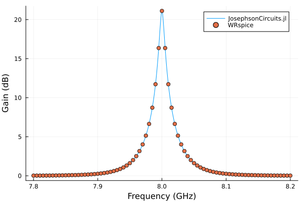

Josephson traveling wave parametric amplifier (JTWPA)

Circuit parameters from here.

using JosephsonCircuits
using Plots

Rleft = 50.0
Rright = 50.0
Cg = 45.0e-15
Lj = IctoLj(3.4e-6)
Cj = 55e-15
Cc = 30.0e-15
Cr = 2.8153e-12
Lr = 1.70e-10

# one unit cell of the line: a junction with its shunt capacitance and
# the capacitance to ground at its input, exposed through pins 1 and 2
jjcell(Lj, Cj, Cg) = Circuit(
    [(:jj, 1, 2, JosephsonJunction(Lj)),
     (:cj, 1, 2, Capacitor(Cj)),
     (:cg, 1, 0, Capacitor(Cg))];
    pins = [1 => (:jj, 1), 2 => (:jj, 2)])

# a cell whose capacitance to ground is split to couple a phase matching
# resonator
pmrcell(Lj, Cj, Cg, Cc, Cr, Lr) = Circuit(
    [(:jj, 1, 2, JosephsonJunction(Lj)),
     (:cj, 1, 2, Capacitor(Cj)),
     (:cg, 1, 0, Capacitor(Cg - Cc)),
     (:cc, 1, 3, Capacitor(Cc)),
     (:cr, 3, 0, Capacitor(Cr)),
     (:lr, 3, 0, Inductor(Lr))];
    pins = [1 => (:jj, 1), 2 => (:jj, 2)])

Nj = 2048
pmrpitch = 4

# instance the cells and chain them: cell i sits between nodes i and i+1
netlist = Any[(:p1, 1, 0, Port(1; Z0 = Rleft))]
for i in 1:Nj-1
    cell = if i == 1
        jjcell(Lj, Cj, Cg/2)             # half cap to ground at the input
    elseif mod(i, pmrpitch) == pmrpitch÷2
        pmrcell(Lj, Cj, Cg, Cc, Cr, Lr)
    else
        jjcell(Lj, Cj, Cg)
    end
    push!(netlist, (Symbol(:cell, i), i, i+1, cell))
end
push!(netlist, (:cend, Nj, 0, Capacitor(Cg/2)))
push!(netlist, (:p2, Nj, 0, Port(2; Z0 = Rright)))

circuit = Circuit(netlist)

ws=2*pi*(1.0:0.1:14)*1e9
wp=(2*pi*7.12*1e9,)
Ip=1.85e-6
sources = [(mode=(1,),port=1,current=Ip)]
Npumpharmonics = (20,)
Nmodulationharmonics = (10,)

@time rpm = hbsolve(ws, wp, sources, Nmodulationharmonics,
    Npumpharmonics, circuit)

p1=plot(ws/(2*pi*1e9),
    10*log10.(abs2.(rpm.linearized.S(
            outputmode=(0,),
            outputport=2,
            inputmode=(0,),
            inputport=1,
            freqindex=:),
    )),
    ylim=(-40,30),label="S21",
    xlabel="Signal Frequency (GHz)",
    legend=:bottomright,
    title="Scattering Parameters",
    ylabel="dB")

plot!(ws/(2*pi*1e9),
    10*log10.(abs2.(rpm.linearized.S((0,),1,(0,),2,:))),
    label="S12",
    )

plot!(ws/(2*pi*1e9),
    10*log10.(abs2.(rpm.linearized.S((0,),1,(0,),1,:))),
    label="S11",
    )

plot!(ws/(2*pi*1e9),
    10*log10.(abs2.(rpm.linearized.S((0,),2,(0,),2,:))),
    label="S22",
    )

p2=plot(ws/(2*pi*1e9),
    rpm.linearized.QE((0,),2,(0,),1,:)./rpm.linearized.QEideal((0,),2,(0,),1,:),
    ylim=(0,1.05),
    title="Quantum efficiency",legend=false,
    ylabel="QE/QE_ideal",xlabel="Signal Frequency (GHz)");

p3=plot(ws/(2*pi*1e9),
    10*log10.(abs2.(rpm.linearized.S(:,2,(0,),1,:)')),
    ylim=(-40,30),
    xlabel="Signal Frequency (GHz)",
    legend=false,
    title="All idlers",
    ylabel="dB")

p4=plot(ws/(2*pi*1e9),
    1 .- rpm.linearized.CM((0,),2,:),
    legend=false,title="Commutation \n relation error",
    ylabel="Commutation \n relation error",xlabel="Signal Frequency (GHz)");

plot(p1, p2, p3, p4, layout = (2, 2))

  2.959010 seconds (257.75 k allocations: 2.392 GiB, 0.21% gc time)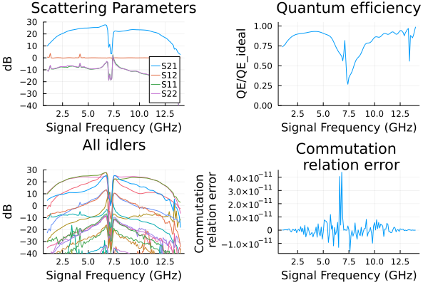

Floquet JTWPA

Circuit parameters from here.

using JosephsonCircuits
using Plots

# a circuit builder: an ordinary function from design parameters to a
# numeric circuit, so parameter changes (like the dielectric loss below)
# are just calls with different keyword arguments
function floquetcircuit(; Rleft = 50.0, Rright = 50.0, Lj = IctoLj(1.75e-6),
    Cg = 76.6e-15, Cc = 40.0e-15, Cr = 1.533e-12, Lr = 2.47e-10, Cj = 40e-15,
    Nj = 2000, pmrpitch = 8, weightwidth = 745)

    weight = (n,Nnodes,weightwidth) -> exp(-(n - Nnodes/2)^2/(weightwidth)^2)

    # the same unit cells as the uniform line, with the junction and
    # capacitance values weighted per cell
    jjcell(Lj, Cj, Cg) = Circuit(
        [(:jj, 1, 2, JosephsonJunction(Lj)),
         (:cj, 1, 2, Capacitor(Cj)),
         (:cg, 1, 0, Capacitor(Cg))];
        pins = [1 => (:jj, 1), 2 => (:jj, 2)])
    pmrcell(Lj, Cj, Cg, Cc, Cr, Lr) = Circuit(
        [(:jj, 1, 2, JosephsonJunction(Lj)),
         (:cj, 1, 2, Capacitor(Cj)),
         (:cg, 1, 0, Capacitor(Cg - Cc)),
         (:cc, 1, 3, Capacitor(Cc)),
         (:cr, 3, 0, Capacitor(Cr)),
         (:lr, 3, 0, Inductor(Lr))];
        pins = [1 => (:jj, 1), 2 => (:jj, 2)])

    # cell i sits between nodes i and i+1
    netlist = Any[(:p1, 1, 0, Port(1; Z0 = Rleft))]
    for i in 1:Nj-1
        wj = weight(i, Nj, weightwidth)
        wg = weight(i - 0.5, Nj, weightwidth)
        cell = if i == 1
            jjcell(Lj*wj, Cj/wj, Cg/2*wg)
        elseif mod(i, pmrpitch) == pmrpitch÷2
            pmrcell(Lj*wj, Cj/wj, Cg*wg, Cc*wg, Cr, Lr)
        else
            jjcell(Lj*wj, Cj/wj, Cg*wg)
        end
        push!(netlist, (Symbol(:cell, i), i, i+1, cell))
    end
    push!(netlist,
        (:cend, Nj, 0, Capacitor(Cg/2*weight(Nj - 0.5, Nj, weightwidth))))
    push!(netlist, (:p2, Nj, 0, Port(2; Z0 = Rright)))

    return Circuit(netlist)
end

circuit = floquetcircuit()

ws=2*pi*(1.0:0.1:14)*1e9
wp=(2*pi*7.9*1e9,)
Ip=1.1e-6
sources = [(mode=(1,),port=1,current=Ip)]
Npumpharmonics = (20,)
Nmodulationharmonics = (10,)

@time floquet = hbsolve(ws, wp, sources, Nmodulationharmonics,
    Npumpharmonics, circuit)

p1=plot(ws/(2*pi*1e9),
    10*log10.(abs2.(floquet.linearized.S((0,),2,(0,),1,:))),
    ylim=(-40,30),label="S21",
    xlabel="Signal Frequency (GHz)",
    legend=:bottomright,
    title="Scattering Parameters",
    ylabel="dB")

plot!(ws/(2*pi*1e9),
    10*log10.(abs2.(floquet.linearized.S((0,),1,(0,),2,:))),
    label="S12",
    )

plot!(ws/(2*pi*1e9),
    10*log10.(abs2.(floquet.linearized.S((0,),1,(0,),1,:))),
    label="S11",
    )

plot!(ws/(2*pi*1e9),
    10*log10.(abs2.(floquet.linearized.S((0,),2,(0,),2,:))),
    label="S22",
    )

p2=plot(ws/(2*pi*1e9),
    floquet.linearized.QE((0,),2,(0,),1,:)./floquet.linearized.QEideal((0,),2,(0,),1,:),
    ylim=(0.99,1.001),
    title="Quantum efficiency",legend=false,
    ylabel="QE/QE_ideal",xlabel="Signal Frequency (GHz)");

p3=plot(ws/(2*pi*1e9),
    10*log10.(abs2.(floquet.linearized.S(:,2,(0,),1,:)')),
    ylim=(-40,30),label="S21",
    xlabel="Signal Frequency (GHz)",
    legend=false,
    title="All idlers",
    ylabel="dB")


p4=plot(ws/(2*pi*1e9),
    1 .- floquet.linearized.CM((0,),2,:),
    legend=false,title="Commutation \n relation error",
    ylabel="Commutation \n relation error",xlabel="Signal Frequency (GHz)");

plot(p1, p2, p3,p4,layout = (2, 2))

  2.079267 seconds (456.63 k allocations: 1.997 GiB, 0.48% gc time)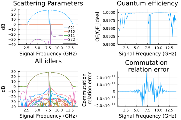

Floquet JTWPA with dissipation

Dissipation due to capacitors with dielectric loss, parameterized by a loss tangent. Run the above code block to define the circuit then run the following:

results = []
tandeltas = [1.0e-6,1.0e-3, 2.0e-3, 3.0e-3]
for tandelta in tandeltas
    # dielectric loss enters through complex capacitances, so build the
    # circuit again with lossy values
    lossycircuit = floquetcircuit(
        Cg = 76.6e-15/(1+im*tandelta),
        Cc = 40.0e-15/(1+im*tandelta),
        Cr = 1.533e-12/(1+im*tandelta),
    )
    wp=(2*pi*7.9*1e9,)
    ws=2*pi*(1.0:0.1:14)*1e9
    Ip=1.1e-6*(1+125*tandelta)
    sources = [(mode=(1,),port=1,current=Ip)]
    Npumpharmonics = (20,)
    Nmodulationharmonics = (10,)
    @time floquet = hbsolve(ws, wp, sources, Nmodulationharmonics,
        Npumpharmonics, lossycircuit)
    push!(results,floquet)
end

p1 = plot(title="Gain (S21)")
for i = 1:length(results)
        plot!(ws/(2*pi*1e9),
            10*log10.(abs2.(results[i].linearized.S((0,),2,(0,),1,:))),
            ylim=(-60,30),label="tanδ=$(tandeltas[i])",
            legend=:bottomleft,
            xlabel="Signal Frequency (GHz)",ylabel="dB")
end

p2 = plot(title="Quantum Efficiency")
for i = 1:length(results)
        plot!(ws/(2*pi*1e9),
            results[i].linearized.QE((0,),2,(0,),1,:)./results[i].linearized.QEideal((0,),2,(0,),1,:),
            ylim=(0.6,1.05),legend=false,
            title="Quantum efficiency",
            ylabel="QE/QE_ideal",xlabel="Signal Frequency (GHz)")
end

p3 = plot(title="Reverse Gain (S12)")
for i = 1:length(results)
        plot!(ws/(2*pi*1e9),
            10*log10.(abs2.(results[i].linearized.S((0,),1,(0,),2,:))),
            ylim=(-10,1),legend=false,
            xlabel="Signal Frequency (GHz)",ylabel="dB")
end

p4 = plot(title="Commutation \n relation error")
for i = 1:length(results)
        plot!(ws/(2*pi*1e9),
            1 .- results[i].linearized.CM((0,),2,:),
            legend=false,
            ylabel="Commutation\n relation error",xlabel="Signal Frequency (GHz)")
end

plot(p1, p2, p3,p4,layout = (2, 2))

  3.815835 seconds (470.00 k allocations: 2.303 GiB, 0.22% gc time)
  3.800166 seconds (470.59 k allocations: 2.310 GiB, 0.29% gc time)
  3.824690 seconds (470.75 k allocations: 2.317 GiB, 0.19% gc time)
  3.838721 seconds (470.75 k allocations: 2.317 GiB, 0.18% gc time)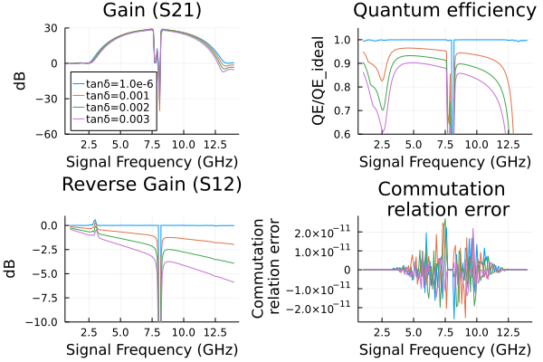

Impedance-engineered JPA

Circuit parameters of the lumped-element snake amplifier (LESA) from here. The device is built from hierarchical subcircuits – a snake stage, a snake, and the four-snake flux-biased SQUID – and its matching network ends in an ideal transmission line expressed directly as a frequency dependent scattering parameter block rather than a discretized LC ladder.

Utility functions

using JosephsonCircuits, Plots

function calc_Lsnake(N,L1,L2,LJ,delta0)
   return N/2*((L1+L2)*LJ+L1*L2*cos(delta0))/(LJ+(4*L1+L2)*cos(delta0))
end

"""
    snakestage(L1, L2, Lj, odd)

One stage of a `snake`: the two arms of the stage -- a Josephson junction
on one and a linear inductor `L2` on the other, swapping arms on
alternating stages -- and the `L1` rung tying the arm outputs together.
Pins 1 and 2 are the arm inputs, pins 3 and 4 the arm outputs.
"""
snakestage(L1, L2, Lj, odd) = Circuit(
    [(:u, 1, 3, odd ? JosephsonJunction(Lj) : Inductor(L2)),
     (:l, 2, 4, odd ? Inductor(L2) : JosephsonJunction(Lj)),
     (:rung, 3, 4, Inductor(L1))];
    pins = [1 => (:u, 1), 2 => (:l, 1), 3 => (:u, 2), 4 => (:l, 2)])

"""
    snake(L1, L2, Lj, Nstages)

A `snake`, a tunable inductor made of two rf-SQUID arrays in parallel as
detailed in arXiv:2209.07757 and PhysRevLett.109.137003: an `L1` rung
across the input, then `Nstages` chained stages.

       <---------Nstages----- ... --->
    1 o--Lj--o--L2--o--Lj- ... -o--L2--o
      |      |      |           |      |
      L1     L1     L1          L1     L1
      |      |      |           |      |
      o--L2--o--Lj--o--L2- ...  o--Lj--o 2

Pin 1 is the start of the upper arm and pin 2 the end of the lower arm.
"""
function snake(L1, L2, Lj, Nstages)
    # the upper and lower arm nodes u1, l1, u2, l2, ... along the snake:
    # stage i spans (ui, li) to (u(i+1), l(i+1))
    netlist = Any[(:rung0, "u1", "l1", Inductor(L1))]
    for i in 1:Nstages
        push!(netlist, (Symbol(:stage, i), "u$i", "l$i", "u$(i+1)", "l$(i+1)",
            snakestage(L1, L2, Lj, isodd(i))))
    end
    return Circuit(netlist;
        pins = [1 => (:stage1, 1), 2 => (Symbol(:stage, Nstages), 4)])
end

"""
    snakesquid(L1, L2, L3, Lj, Lb, K, R, Nstages)

A SQUID made of four `snakes`, flux biased through a port: two arms in
parallel from the single signal pin, each arm two snakes in series
through `L3`, each arm ending in an inductor `Lb` to ground which is
mutually coupled to one of the two bias inductors in series across the
bias port. A positive coupling coefficient adds flux for currents in the
direction the inductors' terminals are declared in, and with both arm
inductors declared toward ground the SQUID loop runs down one arm and up
the other, so the bias current threads the loop through a coupling of
`K` on one arm and `-K` on the other.

    pin 1 o---snake---L3---snake---Lb---gnd   (K to Lb1)
          |
          o---snake---L3---snake---Lb---gnd   (-K to Lb2)

    Port 2 o--R--gnd, with Lb1 and Lb2 in series across it
"""
function snakesquid(L1, L2, L3, Lj, Lb, K, R, Nstages)
    netlist = Any[
        # arm a: node 1 is the signal pin
        (:a1, 1, 2, snake(L1, L2, Lj, Nstages)), (:l3a, 2, 3, Inductor(L3)),
        (:a2, 3, 4, snake(L1, L2, Lj, Nstages)), (:lba, 4, 0, Inductor(Lb)),
        # arm b
        (:b1, 1, 5, snake(L1, L2, Lj, Nstages)), (:l3b, 5, 6, Inductor(L3)),
        (:b2, 6, 7, snake(L1, L2, Lj, Nstages)), (:lbb, 7, 0, Inductor(Lb)),
        # the bias port, with its two inductors in series across it, each
        # coupled to one arm; the loop runs down arm a and up arm b, so the
        # bias current threads it through couplings of opposite sign
        (:p2, 8, 0, Port(2; Z0 = R)),
        (:lb1, 8, 9, Inductor(Lb)), (:lb2, 9, 0, Inductor(Lb)),
        (:kb1, :lba, :lb1, MutualInductor(K)),
        (:kb2, :lbb, :lb2, MutualInductor(-K))]
    return Circuit(netlist; pins = [1 => (:a1, 1)])
end

"""
    tline(theta, w0, Z0)

An ideal transmission line with electrical length `theta` at frequency
`w0` and characteristic impedance `Z0`, as a two port scattering
parameter block: the exact line response, in place of a discretized LC
ladder approximation. The scattering matrix is assembled at each
requested frequency from the ABCD parameters of a line of electrical
length `theta*w/w0`.
"""
function tline(theta, w0, Z0)
    S!(dest, w) = JosephsonCircuits.ABCDtoS!(
        JosephsonCircuits.ABCD_tline!(dest, Z0, theta*w/w0), Z0)
    return ScatteringParameters(S!; nports = 2, zref = Z0, form = :inplace,
        noise = Lossless())
end

LESA simulation

R = 50.0
Lj = JosephsonCircuits.IctoLj(16e-6)
L1 = 2.6e-12
L2 = 8.0e-12
L3 = 5e-12
Lb = 60e-12
K = 0.5*50/sqrt(60*60)
C1 = 6.607e-12
C6 = 0.743e-12
C7 = 0.265e-12
PLCC = 0.654e-12
PLCL = 0.650e-9
L22 = 1.320e-9

Nstages_snake = 10

Z0 = 50.0
w0 = 2*pi*4.9e9
theta = 32.6*pi/180

# the snake SQUID X1 shunts the signal node; C6, the parallel LC, C7 and
# the transmission line -- a scattering parameter block with the exact
# line response -- form the impedance matching network to the port
circuit = Circuit(
    [(:x1, 1, snakesquid(L1, L2, L3, Lj, Lb, K, R, Nstages_snake)),
     (:c1, 1, 0, Capacitor(C1)), (:c6, 1, 2, Capacitor(C6)),
     (:plcc, 2, 0, Capacitor(PLCC)), (:plcl, 2, 0, Inductor(PLCL)),
     (:c7, 2, 3, Capacitor(C7)),
     # a grounded two port block lists the signal node of each port
     (:tl, 3, 4, tline(theta, w0, Z0)),
     (:l22, 4, 0, Inductor(L22)), (:p1, 4, 0, Port(1; Z0 = R))])

# ws = 2*pi*(1:0.01:10.0)*1e9
ws = 2*pi*(4.0:0.01:5.8)*1e9
wp = (2*pi*9.8001*1e9,)
Ip = 0.247e-3
Idc = 0.686e-3
# add the DC bias and pump to port 2
sourcespumpon = [(mode=(0,),port=2,current=Idc),(mode=(1,),port=2,current=Ip)]
Npumpharmonics = (8,)
Nmodulationharmonics = (4,)
@time sol = hbsolve(ws, wp, sourcespumpon, Nmodulationharmonics,
    Npumpharmonics, circuit, dc = true, threewavemixing=true,fourwavemixing=true,
        iterations=200,
)

plot(
    sol.linearized.w/(2*pi*1e9),
    10*log10.(abs2.(
        sol.linearized.S(
            outputmode=(0,),
            outputport=1,
            inputmode=(0,),
            inputport=1,
            freqindex=:
        ),
    )),
    xlabel="Frequency (GHz)",
    ylabel="Gain (dB)",
    label="signal",
    linewidth=2,
    ylim=(-10,30),
#     ylim=(19,22),
#     xlim=(4.69,4.71),
)

plot!(
    sol.linearized.w/(2*pi*1e9),
    10*log10.(abs2.(
        sol.linearized.S(
            outputmode=(-1,),
            outputport=1,
            inputmode=(0,),
            inputport=1,
            freqindex=:
        ).*sqrt.(abs.((wp.-sol.linearized.w)./sol.linearized.w)), # convert from photon number to power
    )),
    linewidth=2,
    xlabel="Frequency (GHz)",
    ylabel="Gain (dB)",
    label="idler",
)

  0.081631 seconds (34.78 k allocations: 67.609 MiB, 48.06% gc time)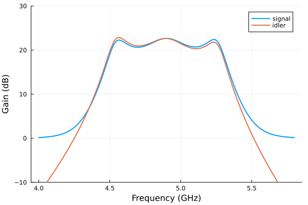

Design parameter sensitivities

The derivative of the scattering parameters with respect to the design parameters of a circuit builder, computed with the adjoint method from a single solve rather than by re-solving per parameter. The builder is an ordinary function from named parameters to a circuit; every component value which depends on a parameter contributes through the chain rule, including derived values.

using JosephsonCircuits
using Plots

makejpa(; Lj, Cc, Cj) = Circuit(
    [(:p1, 1, 0, Port(1)),
     (:cc, 1, 2, Capacitor(Cc)),
     (:jj, 2, 0, JosephsonJunction(Lj)),
     (:cj, 2, 0, Capacitor(Cj))])

p = (Lj = 1000.0e-12, Cc = 100.0e-15, Cj = 1000.0e-15)
ws = 2*pi*(4.5:0.001:5.0)*1e9
wp = (2*pi*4.75001*1e9,)
sources = [(mode=(1,),port=1,current=0.00565e-6)]

@time r = designsensitivities(makejpa, p, ws, wp, sources, (8,), (16,))

# the derivative of the gain in dB with respect to each parameter,
# dG/dp = (20/log(10))*real(conj(S)*dS/dp)/abs2(S), scaled by the
# parameter value so the three curves share units: dB of gain per
# fractional change of the parameter
S = r.out.linearized.S((0,),1,(0,),1,:)
plot(ws/(2*pi*1e9),
    [getproperty(p, q).*(20/log(10)).*
     real.(conj.(S).*r.dSdp((0,),1,(0,),1,q,:))./abs2.(S)
     for q in keys(p)],
    label=["Lj" "Cc" "Cj"],
    xlabel="Frequency (GHz)",
    ylabel="dG/dln(p) (dB)")

Sensitivity to frequency dependent scattering parameters

A ScatteringParameters constructed inside the builder is differentiated like any component value: here a matched transmission line section in front of the amplifier, with the derivative of the gain with respect to the line length. The default is central finite differences through the block's scattering function; this example supplies the analytic derivative through the derivatives keyword instead. A block hoisted out of the builder (measured Touchstone data, say) is treated as parameter independent and costs nothing.

using JosephsonCircuits
using Plots

vphase = 1.2e8 # the phase velocity of the line in m/s
function maketline(; len, Lj)
    # a matched, lossless transmission line: S21 = exp(-im*w*len/vphase)
    tlineS(w) = (t = exp(-im*w*len/vphase); [0 t; t 0])
    # the analytic derivative of S with respect to the length
    dSdlen(w) = (d = -im*w/vphase*exp(-im*w*len/vphase); [0 d; d 0])
    line = ScatteringParameters(tlineS; nports = 2, noise = Lossless(),
        derivatives = (len = dSdlen,))
    return Circuit(
        [(:p1, 1, 0, Port(1)),
         (:tl, 1, 2, line),
         (:cc, 2, 3, Capacitor(100.0e-15)),
         (:jj, 3, 0, JosephsonJunction(Lj)),
         (:c2, 3, 0, Capacitor(1000.0e-15))])
end

p = (len = 2.0e-3, Lj = 1000.0e-12)
ws = 2*pi*(4.5:0.001:5.0)*1e9
wp = (2*pi*4.75001*1e9,)
sources = [(mode=(1,),port=1,current=0.00565e-6)]

@time r = designsensitivities(maketline, p, ws, wp, sources, (8,), (16,))

S = r.out.linearized.S((0,),1,(0,),1,:)
plot(ws/(2*pi*1e9),
    [getproperty(p, q).*(20/log(10)).*
     real.(conj.(S).*r.dSdp((0,),1,(0,),1,q,:))./abs2.(S)
     for q in keys(p)],
    label=["line length" "Lj"],
    xlabel="Frequency (GHz)",
    ylabel="dG/dln(p) (dB)")

Direct current

The harmonic balance state is periodic node flux, and a voltage is its time derivative, so a mode of frequency w has V = i*w*phi0*phi. At zero frequency that is zero, which is right for a capacitor and wrong for a resistor: a resistor would be an open circuit at DC and a current source driving one could not develop I*R.

The solver carries the missing coordinate, the average node voltage, separately. A finite inductor or a zero-voltage Josephson junction has zero average voltage across it, so the average voltage is constant on each connected group of inductors and junctions, and the direct current problem reduces to those coordinates alone. They are carried as a small block of unknowns beside the periodic state, with those equations as their rows, and only when some direct current is injected: with none every average voltage is zero, the periodic system is exact as it stands, and a circuit with no direct current drive pays nothing.

hbnlsolve returns the result as dcnodevoltage, in volts, indexed like nodeflux: ground is excluded, so the first entry is the first real node. It is a vector of zeros when the circuit has a zero frequency mode and no direct current is drawn, and nothing only when the analysis has no zero frequency mode. It is not the same thing as the zero frequency entry of nodeflux, which remains the static periodic flux that sets inductor currents and junction phases.

using JosephsonCircuits

# a current source into a resistor, with a capacitor which carries no
# direct current and an amplifier which is not driven here
Idc = 1.0e-6
circuit = Circuit(
    [(:p1, 1, 0, Port(1; Z0 = 50.0)),
     (:rl, 1, 0, Resistor(150.0)),
     (:c1, 1, 0, Capacitor(1.0e-12))])

sol = hbnlsolve((2*pi*5e9,), (1,), [(mode = (0,), port = 1, current = Idc)],
    circuit; dc = true, odd = true, keyedarrays = false)

# the port environment in parallel with the load, so V = I*(50 || 150)
(sol.dcnodevoltage[1], Idc*inv(1/50.0 + 1/150.0))

(3.749999999999999e-5, 3.75e-5)

An inductor or a junction across a resistor shorts it at DC, so the resistor then carries no direct current however hard it is driven; that is the physical answer rather than a limitation. A resistor between two groups carries current between them, so their average voltages differ by I*R.

Two things are refused rather than approximated. A component whose conductance at zero frequency is not finite and real has no direct current behaviour to use – a frequency dependent resistance whose limit at DC is complex or unbounded, for instance – and is reported with the entry named. And a direct current with nowhere to go, injected into a group of nodes which no resistor, inductor or junction connects to anything else, has no bounded solution and is reported as such before the solve starts.

A scattering block carries direct current according to its zero frequency limit: by default the limit of its own data (ScatteringLimit()), which a constant or tabulated block reaching zero frequency supplies, and otherwise the model stated with its dcmodel keyword, OpenDC(), ShortDC(), ThroughDC() or ScatteringDC(S0). A block whose limit is a short or a through constrains the direct voltages of its ports instead of conducting between them, which the solver handles by an explicit direct current block rather than by the elimination above.