Multi-tone Fourier grids

Each independent strong tone adds an integer coordinate to the HB mode index. For pump frequencies wp, mode m has angular frequency sum(m .* wp). Two or three tones are useful for studying intermodulation; the tensor grid becomes expensive as the number of independent tones grows. Requires JosephsonCircuits and Plots.

A three-tone operating point

This small JPA uses weak drives so that several refinements run quickly. It illustrates the workflow, not a high-gain amplifier design. The three frequencies have no intended common fundamental. For deliberately commensurate drives, use one fundamental and excite its harmonics instead. The three tones drive port 1:

 1                  2
 o------[cc]--------o--------+
 |                  |        |
[p1]              [jj]     [cj]
 |                  |        |
 o------------------o--------+
 0

using JosephsonCircuits, LinearAlgebra, Plots
circuit = Circuit([
    (:p1, 1, 0, Port(1)), (:cc, 1, 2, Capacitor(100e-15)),
    (:jj, 2, 0, JosephsonJunction(1e-9)), (:cj, 2, 0, Capacitor(1e-12)),
])
wp = 2pi .* (4.1e9, sqrt(2)*3.1e9, sqrt(3)*2.9e9)
sources = [(mode = (1,0,0), port = 1, current = 1e-9),
           (mode = (0,1,0), port = 1, current = 1e-9),
           (mode = (0,0,1), port = 1, current = 1e-9)]
function solve_three(; H = (2,2,2), E = (4,4,4), order = 3,
        M = (2,2,2), modulation_order = 2)
    result = hbsolve([2pi*4.7e9], wp, sources, M, H, circuit;
        Nevaluationharmonics = E, maxpumpintermodorder = order,
        maxmodulationintermodorder = modulation_order,
        frequencywindow = (0, 2pi*20e9))
    @assert result.nonlinear.solverinfo.converged
    return result
end
base = solve_three()
S11(result) = result.linearized.S((0,0,0), 1, (0,0,0), 1, 1)
(length(base.nonlinear.modes), S11(base))

(19, 0.6454564279511594 - 0.7637971114686526im)

The source values are Fourier coefficients; each physical cosine has twice that peak current. The modulation index (0,0,0) selects the signal itself. An idler offset m is at ws + sum(m .* wp) and can be negative. See signed frequencies.

Retained modes and conjugate partners

For a real pump waveform, phi[-m] = conj(phi[m]). The nonlinear solve stores one coefficient per conjugate pair. The following panels use the actual retained modes from one-, two-, and three-tone solves, with caps of two on each axis and total intermodulation order at most three. The plotted lattice coordinates are harmonic indices, not frequencies.

grids = [hbnlsolve(wp[1:d], ntuple(_ -> 2, d),
    [(mode = ntuple(k -> Int(k == j), d), port = 1, current = 1e-9)
        for j in 1:d], circuit; maxintermodorder = 3) for d in 1:2]
@assert all(r -> r.solverinfo.converged, grids)
mode_sets = [grids[1].modes, grids[2].modes, base.nonlinear.modes]
panels = map(1:3) do d
    kept = Set(mode_sets[d])
    partners = Set(map(m -> .-m, mode_sets[d]))
    full = vec(collect(Iterators.product(ntuple(_ -> -2:2, d)...)))
    omitted = filter(m -> !(m in kept) && !(m in partners), full)
    p = plot(; title = "$(d) tone$(d == 1 ? "" : "s")", xlabel = "m1",
        ylabel = d == 1 ? "" : "m2", legend = d == 1 ? :topright : false,
        guidefontsize = 10, tickfontsize = 8, titlefontsize = 13,
        xticks = -2:2, yticks = d == 1 ? false : -2:2)
    d == 1 && ylims!(p, -1, 1)
    for (points, color, marker, label) in
            ((omitted, :lightgray, :xcross, "omitted"),
             (collect(partners), :darkorange, :diamond, "conjugate"),
             (collect(kept), :royalblue, :circle, "stored"))
        x = [m[1] for m in points]
        y = d == 1 ? zeros(length(points)) : [m[2] for m in points]
        if d == 3
            scatter!(p, x, y, [m[3] for m in points]; color, marker,
                markersize = 4, label, zlabel = "m3", zticks = -2:2)
        else
            scatter!(p, x, y; color, marker, markersize = 5, label)
        end
    end
    p
end
plot(panels...; layout = (1,3), size = (1000,400),
    bottom_margin = 6 * Plots.mm, left_margin = 4 * Plots.mm)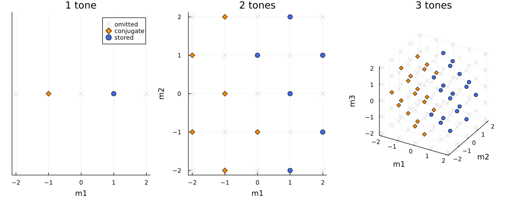

Blue circles are stored coefficients, orange diamonds their conjugates, and gray crosses omitted lattice points. Negative physical frequencies can still occur among stored tuples; the storage convention does not sort by the sign of sum(m .* wp). Linearized signal/idler coordinates have their own mode set; do not halve them by applying the pump's real-wave redundancy a second time.

The default four-wave-mixing pump set has odd sum(m) and excludes DC. An unbiased odd current–phase relation driven at the fundamentals is compatible with that symmetry. A bias or another nonlinearity can require DC and even modes; use the appropriate dc and threewavemixing options. In hbnlsolve the parity options are named odd and even.

Selection	Shape/effect
Npumpharmonics = H	Box: abs(m[j]) <= H[j]
maxpumpintermodorder = q	sum(abs, m) <= q, a diamond in 2D and an octahedron in 3D, and every harmonic of a single tone up to its cap
Parity and DC options	Remove incompatible parity classes or retain the origin
frequencywindow = (lo,hi)	Keep lo <= abs(sum(m .* wp)) <= hi, in rad/s; DC follows dc

The corresponding order keyword of hbnlsolve is maxintermodorder. A frequency floor can remove nearly cancelling combinations on a multi-tone grid, but also removes their physical mixing paths. Refine that cutoff when those low-frequency products matter. Raising only the axis caps adds the harmonics of a single tone, which the order does not cut, but no mixing product the order excludes and no mode outside the frequency window.

Evaluation is a separate grid

The retained coefficients are transformed onto a tensor product of phase samples to evaluate the nonlinear current. Evaluation caps E give 2E[j]+1 samples along each pump phase. These samples are not extra unknown Fourier coefficients, nor are they samples along a single common time period for incommensurate pumps.

The example below shows a two-tone phase torus as a square with periodic edges. Increasing E samples the same retained waveform more densely.

phase_panels = map((2,4)) do E
    phase = 2pi .* (0:2E) ./ (2E + 1)
    scatter(repeat(phase; inner = length(phase)), repeat(phase; outer = length(phase));
        title = "E = ($E,$E): $(length(phase)^2) samples",
        xlabel = "pump phase 1", ylabel = "pump phase 2", legend = false,
        xlims = (-0.15,2pi + 0.15), ylims = (-0.15,2pi + 0.15),
        xticks = ([0,pi,2pi], ["0","π","2π"]),
        yticks = ([0,pi,2pi], ["0","π","2π"]), aspect_ratio = :equal,
        markersize = 3, color = :royalblue)
end
plot(phase_panels...; layout = (1,2), size = (700,380),
    bottom_margin = 6 * Plots.mm, left_margin = 5 * Plots.mm)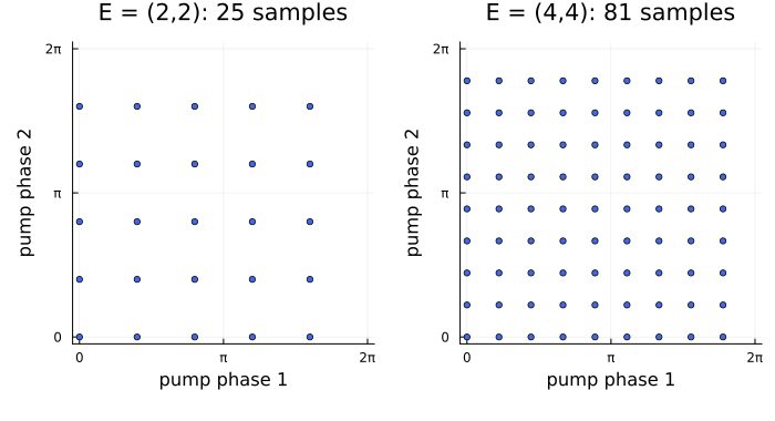

The default E = 2 .* H prevents leading cubic products from aliasing into the retained set. A sine at large phase excursion contains higher orders, so refine evaluation padding separately.

refinements = [
    solve_three(H = (3,3,3), order = 5),  # larger retained pump set, same E
    solve_three(E = (6,6,6)),            # same unknowns, denser evaluation
    solve_three(M = (4,4,4), modulation_order = 4),  # more signal/idler paths
]
changes = [abs(S11(r) - S11(base))/abs(S11(r)) for r in refinements]
@assert maximum(changes) < 1e-3
changes

3-element Vector{Float64}:
 8.345820403304194e-14
 3.2425354985502693e-15
 2.3603664943908676e-15

This checks one response of a weakly driven example. A high-gain device or a weak intermodulation product can need much larger grids. Check those observables directly, along with the nonlinear residual and noise commutator; none of them replaces the other checks.

When to switch to time

Even after a sparse retained-mode cut, nonlinear evaluation uses a full tensor grid. Caps H=(4,4,4) and default E=(8,8,8) need 4913 phase samples per waveform; five such tones need 1,419,857. Factorization, Krylov, and response storage add to the transform buffers. See the memory estimates. For many simultaneous strong tones, consider the ten-signal transient recipe, whose cost instead grows with circuit size, simulated duration, and required time resolution.