

Josephson traveling wave parametric amplifier (JTWPA)
Build a resonant-phase-matched JTWPA from repeated cells. Inspect forward and reverse gain, conversion to idlers, quantum efficiency, and the commutator error. This is a full device example; reduce the cell count for a quick syntax check, but do not expect the same gain.
The plotting code requires Plots in addition to JosephsonCircuits.
Circuit parameters from C. Macklin, K. O'Brien, D. Hover, M. E. Schwartz, V. Bolkhovsky, X. Zhang, W. D. Oliver, and I. Siddiqi, “A near–quantum-limited Josephson traveling-wave parametric amplifier”, Science 350, 307–310 (2015); the harmonic limits are this simulation's. A chain of Nj - 1 cells between two 50 Ω ports, each a junction jj shunted by cj with its capacitance to ground cg at its input; every pmrpitch-th cell couples a resonator, cr and lr, through cc and has Cg - Cc to ground, and the first cell and the end have Cg/2:
 1            2            3                    2048
 o--[cell1]---o--[cell2]---o-- ... --[cell2047]--o
 |                                               |
[p1]                                      [cend || p2]
 |                                               |
 o-----------------------------------------------o
 0

 jjcell                       pmrcell
 1                  2         1                  2
 o---[jj || cj]-----o         o---[jj || cj]-----o
 |                            |
[cg]                          +-------[cc]-------o 3
 |                            |                  |
 o 0                        [cg]           [cr || lr]
                              |                  |
                              o------------------o
0using JosephsonCircuits
using Plots
Rleft = 50.0
Rright = 50.0
Cg = 45.0e-15
Lj = IctoLj(3.4e-6)
Cj = 55e-15
Cc = 30.0e-15
Cr = 2.8153e-12
Lr = 1.70e-10
# one unit cell of the line: a junction with its shunt capacitance and
# the capacitance to ground at its input, exposed through pins 1 and 2
jjcell(Lj, Cj, Cg) = Circuit(
[(:jj, 1, 2, JosephsonJunction(Lj)),
(:cj, 1, 2, Capacitor(Cj)),
(:cg, 1, 0, Capacitor(Cg))];
pins = [1 => (:jj, 1), 2 => (:jj, 2)])
# a cell whose capacitance to ground is split to couple a phase matching
# resonator
pmrcell(Lj, Cj, Cg, Cc, Cr, Lr) = Circuit(
[(:jj, 1, 2, JosephsonJunction(Lj)),
(:cj, 1, 2, Capacitor(Cj)),
(:cg, 1, 0, Capacitor(Cg - Cc)),
(:cc, 1, 3, Capacitor(Cc)),
(:cr, 3, 0, Capacitor(Cr)),
(:lr, 3, 0, Inductor(Lr))];
pins = [1 => (:jj, 1), 2 => (:jj, 2)])
function rpmcircuit(; Nj = 2048, pmrpitch = 4)
# instance the cells and chain them: cell i sits between nodes i and i+1
netlist = Any[(:p1, 1, 0, Port(1; Z0 = Rleft))]
for i in 1:Nj-1
cell = if i == 1
jjcell(Lj, Cj, Cg/2) # half cap to ground at the input
elseif mod(i, pmrpitch) == pmrpitch÷2
pmrcell(Lj, Cj, Cg, Cc, Cr, Lr)
else
jjcell(Lj, Cj, Cg)
end
push!(netlist, (Symbol(:cell, i), i, i+1, cell))
end
push!(netlist, (:cend, Nj, 0, Capacitor(Cg/2)))
push!(netlist, (:p2, Nj, 0, Port(2; Z0 = Rright)))
return Circuit(netlist)
endUse the same builder for the full-size device:
circuit = rpmcircuit()

ws=2*pi*(1.0:0.1:14)*1e9
wp=(2*pi*7.12*1e9,)
Ip=1.85e-6
sources = [(mode=(1,),port=1,current=Ip)]
Npumpharmonics = (20,)
Nmodulationharmonics = (10,)

rpm = hbsolve(ws, wp, sources, Nmodulationharmonics,
    Npumpharmonics, circuit)
@assert rpm.nonlinear.solverinfo.converged

p1=plot(ws/(2*pi*1e9),
    10*log10.(abs2.(rpm.linearized.S(
            outputmode=(0,),
            outputport=2,
            inputmode=(0,),
            inputport=1,
            freqindex=:),
    )),
    ylim=(-40,30),label="S21",
    xlabel="Signal Frequency (GHz)",
    legend=:bottomright,
    title="Scattering Parameters",
    ylabel="dB")

plot!(ws/(2*pi*1e9),
    10*log10.(abs2.(rpm.linearized.S((0,),1,(0,),2,:))),
    label="S12",
    )

plot!(ws/(2*pi*1e9),
    10*log10.(abs2.(rpm.linearized.S((0,),1,(0,),1,:))),
    label="S11",
    )

plot!(ws/(2*pi*1e9),
    10*log10.(abs2.(rpm.linearized.S((0,),2,(0,),2,:))),
    label="S22",
    )

p2=plot(ws/(2*pi*1e9),
    rpm.linearized.QE((0,),2,(0,),1,:)./rpm.linearized.QEideal((0,),2,(0,),1,:),
    ylim=(0,1.05),
    title="Quantum efficiency",legend=false,
    ylabel="QE/QE_ideal",xlabel="Signal Frequency (GHz)");

p3=plot(ws/(2*pi*1e9),
    10*log10.(abs2.(rpm.linearized.S(:,2,(0,),1,:)')),
    ylim=(-40,30),
    xlabel="Signal Frequency (GHz)",
    legend=false,
    title="All idlers",
    ylabel="dB")

p4=plot(ws/(2*pi*1e9),
    1 .- rpm.linearized.CM((0,),2,:),
    legend=false,title="Commutation \n relation error",
    ylabel="Commutation \n relation error",xlabel="Signal Frequency (GHz)");

plot(p1, p2, p3, p4, layout = (2, 2))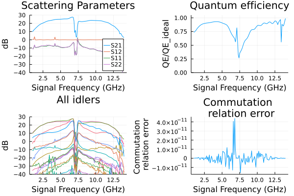
A small executable check
A 32-node version retains several phase-matching resonators and both ports. It checks the builder, pumped solve, and signal/noise outputs. Its gain is not the gain of the full 2048-node line.
small = hbsolve(2pi .* [5e9, 6e9, 8e9], (2pi*7.12e9,),
    [(mode = (1,), port = 1, current = 0.5e-6)], (4,), (8,), rpmcircuit(Nj = 32))
@assert small.nonlinear.solverinfo.converged
@assert all(isfinite, small.linearized.S)
@assert maximum(abs.(abs.(small.linearized.CM) .- 1)) < 1e-5
With the pump off the line is linear, and its transmission is that of the product of its cells' chain matrices: a shunt admittance at each cell's input node, cg and in a resonator cell cc to the resonator, then the junction, its inductance at zero phase in parallel with cj, in series. The solver and the product agree to roundoff, here for the 32-node line and to about 2e-12 for the full one:
series(Z) = [1 Z; 0 1]
shunt(Y) = [1 0; Y 1]
function rpmS21(w; Nj = 2048, pmrpitch = 4)
    junction = series(1/(1/(im*w*Lj) + im*w*Cj))
    resonator = 1/(1/(im*w*Cc) + 1/(im*w*Cr + 1/(im*w*Lr)))
    T = shunt(im*w*Cg/2)*junction
    for i in 2:Nj-1
        Y = mod(i, pmrpitch) == pmrpitch÷2 ? im*w*(Cg - Cc) + resonator : im*w*Cg
        T = T*shunt(Y)*junction
    end
    T = T*shunt(im*w*Cg/2)
    # the transmission between the two 50 ohm ports
    return 2/(T[1, 1] + T[1, 2]/50 + T[2, 1]*50 + T[2, 2])
end
ws = 2pi .* [5e9, 6e9, 8e9]
S21 = hblinsolve(ws, rpmcircuit(Nj = 32)).S((0,), 2, (0,), 1, :)
chain = [rpmS21(w; Nj = 32) for w in ws]
@assert isapprox(S21, chain; atol = 1e-12)
(solver = S21, chain = chain)
(solver = ComplexF64[-0.45026677826718975 - 0.8905369591858728im, -0.7710757356552388 - 0.6350852941150387im, -0.9930307858871927 + 0.11766049661208883im], chain = ComplexF64[-0.4502667782671873 - 0.8905369591858745im, -0.7710757356552195 - 0.6350852941150623im, -0.9930307858871935 + 0.11766049661207653im])