Impedance-engineered JPA

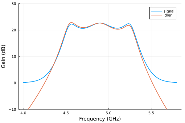
Build an impedance-engineered JPA from nested snake and SQUID subcircuits. The signal and conjugate-idler curves are plotted in power units, so the idler conversion includes the absolute frequency ratio.

The plotting code requires Plots in addition to JosephsonCircuits.

Circuit parameters of the lumped-element snake amplifier (LESA) from Naaman et al. (2024). The device is built from hierarchical subcircuits – a snake stage, a snake, and the four-snake flux-biased SQUID – and its matching network ends in an ideal TransmissionLine rather than a discretized LC ladder.

The snake SQUID x1, flux biased and pumped through its own port 2, shunts node 1; c6, the parallel plcc and plcl, c7, the line tl and l22 match it to port 1:

text

 1          2                  3                 4
 o---[c6]---o-------[c7]-------o------[tl]-------o
 |          |                                    |
[x1 || c1] [plcc || plcl]                  [l22 || p1]
 |          |                                    |
 o----------o------------------------------------o
 0

Utility functions

julia

using JosephsonCircuits

"""
    snakestage(L1, L2, Lj, odd)

One stage of a `snake`: the two arms of the stage -- a Josephson junction
on one and a linear inductor `L2` on the other, swapping arms on
alternating stages -- and the `L1` rung tying the arm outputs together.
Pins 1 and 2 are the arm inputs, pins 3 and 4 the arm outputs.
"""
snakestage(L1, L2, Lj, odd) = Circuit(
    [(:u, 1, 3, odd ? JosephsonJunction(Lj) : Inductor(L2)),
     (:l, 2, 4, odd ? Inductor(L2) : JosephsonJunction(Lj)),
     (:rung, 3, 4, Inductor(L1))];
    pins = [1 => (:u, 1), 2 => (:l, 1), 3 => (:u, 2), 4 => (:l, 2)])

"""
    snake(L1, L2, Lj, Nstages)

A `snake`, a tunable inductor made of two rf-SQUID arrays in parallel as
detailed in arXiv:2209.07757 and PhysRevLett.109.137003: an `L1` rung
across the input, then `Nstages` chained stages.

       <---------Nstages----- ... --->
    1 o--Lj--o--L2--o--Lj- ... -o--L2--o
      |      |      |           |      |
      L1     L1     L1          L1     L1
      |      |      |           |      |
      o--L2--o--Lj--o--L2- ...  o--Lj--o 2

Pin 1 is the start of the upper arm and pin 2 the end of the lower arm.
"""
function snake(L1, L2, Lj, Nstages)
    # the upper and lower arm nodes u1, l1, u2, l2, ... along the snake:
    # stage i spans (ui, li) to (u(i+1), l(i+1))
    netlist = Any[(:rung0, "u1", "l1", Inductor(L1))]
    for i in 1:Nstages
        push!(netlist, (Symbol(:stage, i), "u$i", "l$i", "u$(i+1)", "l$(i+1)",
            snakestage(L1, L2, Lj, isodd(i))))
    end
    return Circuit(netlist;
        pins = [1 => (:stage1, 1), 2 => (Symbol(:stage, Nstages), 4)])
end

"""
    snakesquid(L1, L2, L3, Lj, Lb, K, R, Nstages)

A SQUID made of four `snakes`, flux biased through a port: two arms in
parallel from the single signal pin, each arm two snakes in series
through `L3`, each arm ending in an inductor `Lb` to ground which is
mutually coupled to one of the two bias inductors in series across the
bias port. A positive coupling coefficient adds flux for currents in the
direction the inductors' terminals are declared in, and with both arm
inductors declared toward ground the SQUID loop runs down one arm and up
the other, so the bias current threads the loop through a coupling of
`K` on one arm and `-K` on the other.

    pin 1 o---snake---L3---snake---Lb---gnd   (K to Lb1)
          |
          o---snake---L3---snake---Lb---gnd   (-K to Lb2)

    Port 2 o--R--gnd, with Lb1 and Lb2 in series across it
"""
function snakesquid(L1, L2, L3, Lj, Lb, K, R, Nstages)
    netlist = Any[
        # arm a: node 1 is the signal pin
        (:a1, 1, 2, snake(L1, L2, Lj, Nstages)), (:l3a, 2, 3, Inductor(L3)),
        (:a2, 3, 4, snake(L1, L2, Lj, Nstages)), (:lba, 4, 0, Inductor(Lb)),
        # arm b
        (:b1, 1, 5, snake(L1, L2, Lj, Nstages)), (:l3b, 5, 6, Inductor(L3)),
        (:b2, 6, 7, snake(L1, L2, Lj, Nstages)), (:lbb, 7, 0, Inductor(Lb)),
        # the bias port, with its two inductors in series across it, each
        # coupled to one arm; the loop runs down arm a and up arm b, so the
        # bias current threads it through couplings of opposite sign
        (:p2, 8, 0, Port(2; Z0 = R)),
        (:lb1, 8, 9, Inductor(Lb)), (:lb2, 9, 0, Inductor(Lb)),
        (:kb1, :lba, :lb1, MutualInductor(K)),
        (:kb2, :lbb, :lb2, MutualInductor(-K))]
    return Circuit(netlist; pins = [1 => (:a1, 1)])
end

LESA simulation

julia

R = 50.0
Lj = JosephsonCircuits.IctoLj(16e-6)
L1 = 2.6e-12
L2 = 8.0e-12
L3 = 5e-12
Lb = 60e-12
K = 0.5*50/sqrt(60*60)
C1 = 6.607e-12
C6 = 0.743e-12
C7 = 0.265e-12
PLCC = 0.654e-12
PLCL = 0.650e-9
L22 = 1.320e-9

Nstages_snake = 10

Z0 = 50.0
w0 = 2*pi*4.9e9
theta = 32.6*pi/180
# the length of a line of electrical length theta at w0
len = theta*JosephsonCircuits.speed_of_light/w0

# the snake SQUID X1 shunts the signal node; C6, the parallel LC, C7 and
# the transmission line form the impedance matching network to the port
circuit = Circuit(
    [(:x1, 1, snakesquid(L1, L2, L3, Lj, Lb, K, R, Nstages_snake)),
     (:c1, 1, 0, Capacitor(C1)), (:c6, 1, 2, Capacitor(C6)),
     (:plcc, 2, 0, Capacitor(PLCC)), (:plcl, 2, 0, Inductor(PLCL)),
     (:c7, 2, 3, Capacitor(C7)),
     # a grounded two port block lists the signal node of each port
     (:tl, 3, 4, TransmissionLine(Z0, len)),
     (:l22, 4, 0, Inductor(L22)), (:p1, 4, 0, Port(1; Z0 = R))])
wp = (2*pi*9.8001*1e9,)
Ip = 0.247e-3
Idc = 0.686e-3
# add the DC bias and pump to port 2
sourcespumpon = [(mode=(0,),port=2,current=Idc),(mode=(1,),port=2,current=Ip)]
Npumpharmonics = (8,)
Nmodulationharmonics = (4,)

The sweep and its plot:

julia

using Plots
ws = 2*pi*(4.0:0.01:5.8)*1e9
sol = hbsolve(ws, wp, sourcespumpon, Nmodulationharmonics,
    Npumpharmonics, circuit, dc = true, threewavemixing=true,fourwavemixing=true,
        iterations=200,
)
@assert sol.nonlinear.solverinfo.converged

plot(
    sol.linearized.w/(2*pi*1e9),
    10*log10.(abs2.(
        sol.linearized.S(
            outputmode=(0,),
            outputport=1,
            inputmode=(0,),
            inputport=1,
            freqindex=:
        ),
    )),
    xlabel="Frequency (GHz)",
    ylabel="Gain (dB)",
    label="signal",
    linewidth=2,
    ylim=(-10,30),
)

plot!(
    sol.linearized.w/(2*pi*1e9),
    10*log10.(abs2.(
        sol.linearized.S(
            outputmode=(-1,),
            outputport=1,
            inputmode=(0,),
            inputport=1,
            freqindex=:
        ).*sqrt.(abs.((wp.-sol.linearized.w)./sol.linearized.w)), # convert from photon number to power
    )),
    linewidth=2,
    xlabel="Frequency (GHz)",
    ylabel="Gain (dB)",
    label="idler",
)

A small executable check

With the pump and the bias off the circuit is linear, and its reflection has a closed form. Each snake is an inductance, its ladder of L1, L2 and junction inductances solved by nodal analysis below; the two arms of the SQUID carry equal currents, whose couplings to the bias inductors, K and -K, cancel, so the SQUID is the inductance (2Lsnake + L3 + Lb)/2, and the matching network and the line take it to port 1:

julia

# the inductance between the pins of a snake: its 2N + 2 arm nodes, the
# far pin the reference
function snakeinductance(L1, L2, Lj, N)
    u(i) = i
    l(i) = N + 1 + i
    G = zeros(2N + 2, 2N + 2)
    add!(a, b, L) = (G[a, a] += 1/L; G[b, b] += 1/L; G[a, b] -= 1/L; G[b, a] -= 1/L)
    add!(u(1), l(1), L1)
    for i in 1:N
        add!(u(i), u(i + 1), isodd(i) ? Lj : L2)
        add!(l(i), l(i + 1), isodd(i) ? L2 : Lj)
        add!(u(i + 1), l(i + 1), L1)
    end
    return (G[1:2N + 1, 1:2N + 1] \ [1.0; zeros(2N)])[1]
end
Lsquid = (2snakeinductance(L1, L2, Lj, Nstages_snake) + L3 + Lb)/2
function reflection(w)
    Z = 1/(1/(im*w*Lsquid) + im*w*C1) + 1/(im*w*C6)
    Z = 1/(1/Z + im*w*PLCC + 1/(im*w*PLCL)) + 1/(im*w*C7)
    t = tan(theta*w/w0)
    Z = Z0*(Z + im*Z0*t)/(Z0 + im*Z*t)
    Z = 1/(1/Z + 1/(im*w*L22))
    return (Z - R)/(Z + R)
end
ws = 2pi .* [4.6e9, 4.9e9, 5.2e9]
S11 = hblinsolve(ws, circuit).S((0,), 1, (0,), 1, :)
@assert isapprox(S11, reflection.(ws); atol = 1e-11)
(solver = S11, closed = reflection.(ws))

(solver = ComplexF64[-0.9990206456140069 + 0.04424646468332559im, 0.22124432637492064 + 0.9752184104327142im, 0.9420142438822318 + 0.3355728897318564im], closed = ComplexF64[-0.9990206456140324 + 0.04424646468275208im, 0.2212443263744777 + 0.9752184104328135im, 0.9420142438820712 + 0.33557288973230553im])

The pumped solve at the same frequencies:

julia

pumped = hbsolve(ws, wp, sourcespumpon, Nmodulationharmonics,
    Npumpharmonics, circuit; dc = true, threewavemixing = true,
    fourwavemixing = true, iterations = 200)
@assert pumped.nonlinear.solverinfo.converged
@assert maximum(abs.(abs.(pumped.linearized.CM) .- 1)) < 1e-8
round.(10 .* log10.(abs2.(pumped.linearized.S((0,), 1, (0,), 1, :))); digits = 2)

1-dimensional KeyedArray(NamedDimsArray(...)) with keys:
↓   freqindex ∈ 3-element UnitRange{Int64}
And data, 3-element Vector{Float64}:
 (1)  21.77
 (2)  22.76
 (3)  21.89

Impedance-engineered JPA ​

A small executable check ​

Impedance-engineered JPA

A small executable check