

Floquet JTWPA
Taper the unit-cell parameters of a traveling-wave amplifier, then add dielectric loss. The second section reuses floquetcircuit from the first. Compare gain and normalized quantum efficiency; refine the harmonic limits as the harmonic balance guide describes before relying on either.
The plotting code requires Plots in addition to JosephsonCircuits.
Gain and HB convergence do not establish temporal stability. Use the pole-analysis workflow to search about a converged periodic solution, refine harmonics, and inspect mode profiles. The constant complex dielectric-loss values used below are frequency-domain models: replace them with an appropriate causal model and recompute the HB orbit before applying hbstability.
Circuit parameters from K. Peng, M. Naghiloo, J. Wang, G. D. Cunningham, Y. Ye, and K. P. O'Brien, “Floquet-mode traveling-wave parametric amplifiers”, PRX Quantum 3, 020306 (2022). The harmonic limits, the loss tangents of the second section and the pump current raised with them are this simulation's. The cells of the JTWPA, jjcell and pmrcell, with their junction inductance, junction capacitance and capacitances to ground and to the resonators weighted along the line by a Gaussian taper:
 1            2                       2000
 o--[cell1]---o-- ... --[cell1999]-----o
 |                                     |
[p1]                            [cend || p2]
 |                                     |
 o-------------------------------------o
0using JosephsonCircuits
using Plots
# a circuit builder: an ordinary function from design parameters to a
# numeric circuit, so parameter changes (like the dielectric loss below)
# are just calls with different keyword arguments
function floquetcircuit(; Rleft = 50.0, Rright = 50.0, Lj = IctoLj(1.75e-6),
Cg = 76.6e-15, Cc = 40.0e-15, Cr = 1.533e-12, Lr = 2.47e-10, Cj = 40e-15,
Nj = 2000, pmrpitch = 8, weightwidth = 745)
weight = (n,Nnodes,weightwidth) -> exp(-(n - Nnodes/2)^2/(weightwidth)^2)
# the same unit cells as the uniform line, with the junction and
# capacitance values weighted per cell
jjcell(Lj, Cj, Cg) = Circuit(
[(:jj, 1, 2, JosephsonJunction(Lj)),
(:cj, 1, 2, Capacitor(Cj)),
(:cg, 1, 0, Capacitor(Cg))];
pins = [1 => (:jj, 1), 2 => (:jj, 2)])
pmrcell(Lj, Cj, Cg, Cc, Cr, Lr) = Circuit(
[(:jj, 1, 2, JosephsonJunction(Lj)),
(:cj, 1, 2, Capacitor(Cj)),
(:cg, 1, 0, Capacitor(Cg - Cc)),
(:cc, 1, 3, Capacitor(Cc)),
(:cr, 3, 0, Capacitor(Cr)),
(:lr, 3, 0, Inductor(Lr))];
pins = [1 => (:jj, 1), 2 => (:jj, 2)])
# cell i sits between nodes i and i+1
netlist = Any[(:p1, 1, 0, Port(1; Z0 = Rleft))]
for i in 1:Nj-1
wj = weight(i, Nj, weightwidth)
wg = weight(i - 0.5, Nj, weightwidth)
cell = if i == 1
jjcell(Lj*wj, Cj/wj, Cg/2*wg)
elseif mod(i, pmrpitch) == pmrpitch÷2
pmrcell(Lj*wj, Cj/wj, Cg*wg, Cc*wg, Cr, Lr)
else
jjcell(Lj*wj, Cj/wj, Cg*wg)
end
push!(netlist, (Symbol(:cell, i), i, i+1, cell))
end
push!(netlist,
(:cend, Nj, 0, Capacitor(Cg/2*weight(Nj - 0.5, Nj, weightwidth))))
push!(netlist, (:p2, Nj, 0, Port(2; Z0 = Rright)))
return Circuit(netlist)
endThe full-size calculation uses that builder:
circuit = floquetcircuit()

ws=2*pi*(1.0:0.1:14)*1e9
wp=(2*pi*7.9*1e9,)
Ip=1.1e-6
sources = [(mode=(1,),port=1,current=Ip)]
Npumpharmonics = (20,)
Nmodulationharmonics = (10,)

floquet = hbsolve(ws, wp, sources, Nmodulationharmonics,
    Npumpharmonics, circuit)
@assert floquet.nonlinear.solverinfo.converged

p1=plot(ws/(2*pi*1e9),
    10*log10.(abs2.(floquet.linearized.S((0,),2,(0,),1,:))),
    ylim=(-40,30),label="S21",
    xlabel="Signal Frequency (GHz)",
    legend=:bottomright,
    title="Scattering Parameters",
    ylabel="dB")

plot!(ws/(2*pi*1e9),
    10*log10.(abs2.(floquet.linearized.S((0,),1,(0,),2,:))),
    label="S12",
    )

plot!(ws/(2*pi*1e9),
    10*log10.(abs2.(floquet.linearized.S((0,),1,(0,),1,:))),
    label="S11",
    )

plot!(ws/(2*pi*1e9),
    10*log10.(abs2.(floquet.linearized.S((0,),2,(0,),2,:))),
    label="S22",
    )

p2=plot(ws/(2*pi*1e9),
    floquet.linearized.QE((0,),2,(0,),1,:)./floquet.linearized.QEideal((0,),2,(0,),1,:),
    ylim=(0.99,1.001),
    title="Quantum efficiency",legend=false,
    ylabel="QE/QE_ideal",xlabel="Signal Frequency (GHz)");

p3=plot(ws/(2*pi*1e9),
    10*log10.(abs2.(floquet.linearized.S(:,2,(0,),1,:)')),
    ylim=(-40,30),label="S21",
    xlabel="Signal Frequency (GHz)",
    legend=false,
    title="All idlers",
    ylabel="dB")

p4=plot(ws/(2*pi*1e9),
    1 .- floquet.linearized.CM((0,),2,:),
    legend=false,title="Commutation \n relation error",
    ylabel="Commutation \n relation error",xlabel="Signal Frequency (GHz)");

plot(p1, p2, p3,p4,layout = (2, 2))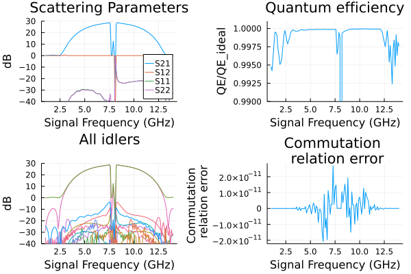
Floquet JTWPA with dissipation
Dissipation due to capacitors with dielectric loss, parameterized by a loss tangent. Run the above code block to define the circuit then run the following:
results = []
tandeltas = [1.0e-6,1.0e-3, 2.0e-3, 3.0e-3]
for tandelta in tandeltas
    # dielectric loss enters through complex capacitances, so build the
    # circuit again with lossy values
    lossycircuit = floquetcircuit(
        Cg = 76.6e-15/(1+im*tandelta),
        Cc = 40.0e-15/(1+im*tandelta),
        Cr = 1.533e-12/(1+im*tandelta),
    )
    wp=(2*pi*7.9*1e9,)
    ws=2*pi*(1.0:0.1:14)*1e9
    Ip=1.1e-6*(1+125*tandelta)
    sources = [(mode=(1,),port=1,current=Ip)]
    Npumpharmonics = (20,)
    Nmodulationharmonics = (10,)
    floquet = hbsolve(ws, wp, sources, Nmodulationharmonics,
        Npumpharmonics, lossycircuit)
    @assert floquet.nonlinear.solverinfo.converged
    push!(results,floquet)
end

p1 = plot(title="Gain (S21)")
for i = 1:length(results)
        plot!(ws/(2*pi*1e9),
            10*log10.(abs2.(results[i].linearized.S((0,),2,(0,),1,:))),
            ylim=(-60,30),label="tanδ=$(tandeltas[i])",
            legend=:bottomleft,
            xlabel="Signal Frequency (GHz)",ylabel="dB")
end

p2 = plot(title="Quantum Efficiency")
for i = 1:length(results)
        plot!(ws/(2*pi*1e9),
            results[i].linearized.QE((0,),2,(0,),1,:)./results[i].linearized.QEideal((0,),2,(0,),1,:),
            ylim=(0.6,1.05),legend=false,
            title="Quantum efficiency",
            ylabel="QE/QE_ideal",xlabel="Signal Frequency (GHz)")
end

p3 = plot(title="Reverse Gain (S12)")
for i = 1:length(results)
        plot!(ws/(2*pi*1e9),
            10*log10.(abs2.(results[i].linearized.S((0,),1,(0,),2,:))),
            ylim=(-10,1),legend=false,
            xlabel="Signal Frequency (GHz)",ylabel="dB")
end

p4 = plot(title="Commutation \n relation error")
for i = 1:length(results)
        plot!(ws/(2*pi*1e9),
            1 .- results[i].linearized.CM((0,),2,:),
            legend=false,
            ylabel="Commutation\n relation error",xlabel="Signal Frequency (GHz)")
end

plot(p1, p2, p3,p4,layout = (2, 2))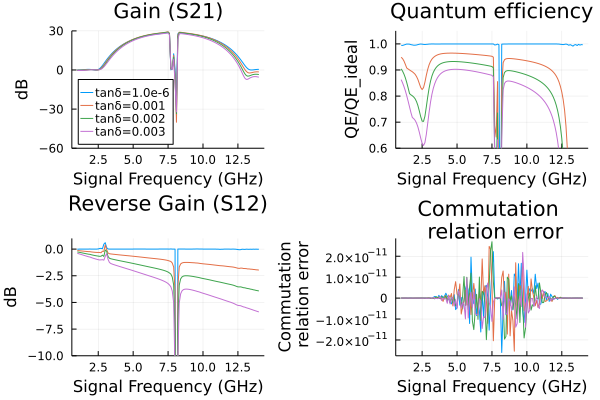
A small executable check
The documentation build exercises the same tapered circuit at 32 nodes, including the dielectric-loss variant. The shorter taper and weaker pump are checks of the recipe, not a substitute for convergence and stability analysis of the full device. With the pump off the line is linear, and its transmission is that of the product of its cells' chain matrices, as for the JTWPA, with the tapered values; the solver and the product agree to roundoff, lossless and lossy, here for the 32-node line and to about 2e-13 for the full one.
series(Z) = [1 Z; 0 1]
shunt(Y) = [1 0; Y 1]
function floquetS21(w; Lj = IctoLj(1.75e-6), Cg = 76.6e-15, Cc = 40.0e-15,
        Cr = 1.533e-12, Lr = 2.47e-10, Cj = 40e-15, Nj = 2000, pmrpitch = 8,
        weightwidth = 745)
    weight(n) = exp(-(n - Nj/2)^2/weightwidth^2)
    T = series(0)
    for i in 1:Nj-1
        wj, wg = weight(i), weight(i - 0.5)
        Y = if i == 1
            im*w*Cg/2*wg
        elseif mod(i, pmrpitch) == pmrpitch÷2
            im*w*(Cg - Cc)*wg + 1/(1/(im*w*Cc*wg) + 1/(im*w*Cr + 1/(im*w*Lr)))
        else
            im*w*Cg*wg
        end
        T = T*shunt(Y)*series(1/(1/(im*w*Lj*wj) + im*w*Cj/wj))
    end
    T = T*shunt(im*w*Cg/2*weight(Nj - 0.5))
    # the transmission between the two 50 ohm ports
    return 2/(T[1, 1] + T[1, 2]/50 + T[2, 1]*50 + T[2, 2])
end
ws = 2pi .* [5e9, 6e9, 9e9]
checks = map((0.0, 1e-3)) do tandelta
    values = (Nj = 32, weightwidth = 12, Cg = 76.6e-15/(1 + im*tandelta),
        Cc = 40e-15/(1 + im*tandelta), Cr = 1.533e-12/(1 + im*tandelta))
    smallcircuit = floquetcircuit(; values...)
    small = hbsolve(ws, (2pi*7.9e9,),
        [(mode = (1,), port = 1, current = 0.3e-6)], (4,), (8,), smallcircuit)
    @assert small.nonlinear.solverinfo.converged
    @assert all(isfinite, small.linearized.S)
    @assert all(isfinite, small.linearized.QE)
    @assert maximum(abs.(abs.(small.linearized.CM) .- 1)) < 1e-5
    S21 = hblinsolve(ws, smallcircuit).S((0,), 2, (0,), 1, :)
    chain = [floquetS21(w; values...) for w in ws]
    @assert isapprox(S21, chain; atol = 1e-12)
    (tandelta = tandelta, difference = maximum(abs.(S21 .- chain)))
end
((tandelta = 0.0, difference = 3.734762037113937e-14), (tandelta = 0.001, difference = 3.821687773350981e-14))